---
title: "Working with big data"
subtitle: "Programming for Statistical Science"
author: "Shawn Santo"
institute: ""
date: ""
output:
xaringan::moon_reader:
css: "slides.css"
lib_dir: libs
nature:
highlightStyle: github
highlightLines: true
countIncrementalSlides: false
editor_options:
chunk_output_type: console
---
```{r include=FALSE}
knitr::opts_chunk$set(echo = TRUE, message = FALSE, warning = FALSE,
comment = "#>", highlight = TRUE,
fig.align = "center")
```
## Supplementary materials
Full video lecture available in Zoom Cloud Recordings
Additional resources
- [Chapter 2](https://adv-r.hadley.nz/names-values.html), Advanced R by Wickham, H.
- `vroom` [vignette](https://cran.r-project.org/web/packages/vroom/vignettes/vroom.html)
---
class: inverse, center, middle
# Memory basics
---
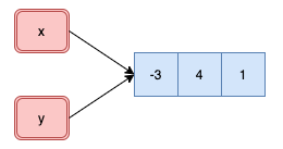
## Names and values
In R, a name has a value. It is not the value that has a name.
For example, in
```{r}
x <- c(-3, 4, 1)
```
the object named `x` is a reference to vector `c(-3, 4, 1)`.
 ---
We can see where this lives in memory with
```{r}
library(lobstr)
lobstr::obj_addr(x)
```
and its size with
```{r}
lobstr::obj_size(x)
```
---
## Copy-on-modify: atomic vectors
Understanding when R creates a copy of an object will allow you to write
faster code. This is also important to keep in mind when working with very
large vectors.
```{r}
x <- c(-3, 4, 1)
y <- x
```
--
```{r}
obj_addr(x)
obj_addr(y)
```
---
We can see where this lives in memory with
```{r}
library(lobstr)
lobstr::obj_addr(x)
```
and its size with
```{r}
lobstr::obj_size(x)
```
---
## Copy-on-modify: atomic vectors
Understanding when R creates a copy of an object will allow you to write
faster code. This is also important to keep in mind when working with very
large vectors.
```{r}
x <- c(-3, 4, 1)
y <- x
```
--
```{r}
obj_addr(x)
obj_addr(y)
```
 ---
```{r}
y[3] <- 100
```
--
```{r}
obj_addr(x)
obj_addr(y)
```
---
```{r}
y[3] <- 100
```
--
```{r}
obj_addr(x)
obj_addr(y)
```
 ---
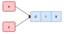
.pull-left[
```{r}
x <- c(0, 1, 9)
y <- x
obj_addr(x)
obj_addr(y)
```
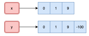
```{r}
y[4] <- -100
obj_addr(x)
obj_addr(y)
```
]
.pull-right[
---
.pull-left[
```{r}
x <- c(0, 1, 9)
y <- x
obj_addr(x)
obj_addr(y)
```
```{r}
y[4] <- -100
obj_addr(x)
obj_addr(y)
```
]
.pull-right[
 ]
]
--
Even though only one component changed in the atomic vector `y`, R created
a new object as seen by the new address in memory.
???
## Copy-on-modify and loops
Poor loop implementation
.tiny[
```{r eval=FALSE}
n <- 8
x <- 1
for (i in seq_len(n)) {
cat("Object address start iteration", i, ":", obj_addr(x), "\n")
x <- c(x, sqrt(x[i] * i))
cat("Object address end iteration ", i, ":", obj_addr(x), "\n\n")
}
```
]
"Efficient" loop implementation
.tiny[
```{r eval=FALSE}
n <- 8
x <- rep(1, n + 1)
ref(x)
for (i in seq_len(n)) {
cat("Object address start iteration", i, ":", ref(x), "\n")
x[i + 1] <- mean(x[i] * i)
cat("Object address end iteration ", i, ":", ref(x), "\n\n")
}
```
]
---
## Memory tracking
Function `tracemem()` marks an object so that a message is printed whenever the
internal code copies the object. Let's see when `x` gets copied.
```{r}
x <- c(0, 1, 1, 2, 3, 5, 8, 13, 21, 34)
tracemem(x)
```
--
```{r}
y <- x
```
--
```{r}
y[1] <- 0
```
---
```{r}
x
y
c(obj_addr(x), obj_addr(y))
```
--
```{r}
x[1] <- 0
```
--
```{r}
lobstr::ref(x)
lobstr::ref(y)
untracemem(x)
```
---
## Copy-on-modify: lists
```{r}
x <- list(a = 1, b = 2, c = 3)
obj_addr(x)
```
--
```{r}
y <- x
```
--
```{r}
c(obj_addr(x), obj_addr(y))
```
--
```{r}
ref(x, y)
```
---
```{r}
y$c <- 4
```
--
```{r}
ref(x, y)
```
---
```{r}
x <- list(a = 1, b = 2, c = 3)
y <- x
```
--
```{r}
c(obj_addr(x), obj_addr(y))
```
--
```{r}
y$d <- 9
ref(x, y)
```
R creates a shallow copy. Shared components exist with elements `a`, `b`, and
`c`.
---
## Copy-on-modify: data frames
```{r}
library(tidyverse)
x <- tibble(a = 1:3, b = 9:7)
```
--
```{r}
ref(x)
```
--
```{r}
y <- x %>%
mutate(b = b ^ 2)
```
--
```{r}
ref(x, y)
```
---
```{r}
z <- x
ref(x, z)
```
--
```{r}
z <- x %>%
add_row(a = -1, b = -1)
```
--
```{r}
ref(x, z)
```
--
If you modify a column, only that column needs to be copied in memory. However,
if you modify a row, the entire data frame is copied in memory.
---
## Exercise
Can you diagnose what is going on below?
```{r}
x <- 1:10; y <- x;
tracemem(x)
c(obj_addr(x), obj_addr(y))
y[1] <- 3
```
---
## Object size
Object sizes can sometimes be deceiving.
```{r}
x <- rnorm(1e6)
y <- 1:1e6
z <- seq(1, 1e6, by = 1)
s <- (1:1e6) / 2
```
--
```{r}
c(obj_size(x), obj_size(y), obj_size(z), obj_size(s))
```
---
```{r}
c(obj_size(c(1L)), obj_size(c(1.0)))
```
--
```{r}
c(obj_size(c(1L, 2L)), obj_size(as.numeric(c(1.0, 2.0))))
```
--
```{r}
c(obj_size(c(1L, 2L, 3L)), obj_size(as.numeric(c(1.0, 2.0, 3.0))))
```
--
```{r}
c(obj_size(integer(10000)), obj_size(numeric(10000)))
```
--
There is overhead with creating vectors in R. Take a look at `?Memory` if
you want to dig deeper as to the overhead cost.
---
## Exercise
Starting from 0 we can see that
```{r}
lobstr::obj_size(integer(0))
lobstr::obj_size(numeric(0))
```
are both 48 bytes. Based on the results on the next slide can you deduce how
R handles these numeric data in memory?
---
```{r}
diff(sapply(0:100, function(x) lobstr::obj_size(integer(x))))
```
```{r}
c(obj_size(integer(20)), obj_size(integer(22)))
```
```{r}
diff(sapply(0:100, function(x) lobstr::obj_size(numeric(x))))
```
```{r}
c(obj_size(numeric(10)), obj_size(numeric(14)))
```
---
class: inverse, center, middle
# I/O big data
---
## Getting big data into R
Dimensions: 3,185,906 x 9
```{r}
url <- "http://www2.stat.duke.edu/~sms185/data/bike/cbs_2015.csv"
```
.tiny[
```{r eval=FALSE}
system.time({x <- read.csv(url)})
```
```{r eval=FALSE}
user system elapsed
*29.739 1.085 37.321
```
]
--
.tiny[
```{r eval=FALSE}
system.time({x <- readr::read_csv(url)})
```
```{r eval=FALSE}
Parsed with column specification:
cols(
Duration = col_double(),
`Start date` = col_datetime(format = ""),
`End date` = col_datetime(format = ""),
`Start station number` = col_double(),
`Start station` = col_character(),
`End station number` = col_double(),
`End station` = col_character(),
`Bike number` = col_character(),
`Member type` = col_character()
)
|================================| 100% 369 MB
user system elapsed
*12.773 1.727 22.327
```
]
---
.tiny[
```{r eval=FALSE}
system.time({x <- data.table::fread(url)})
```
```{r eval=FALSE}
trying URL 'http://www2.stat.duke.edu/~sms185/data/bike/cbs_2015.csv'
Content type 'text/csv' length 387899567 bytes (369.9 MB)
==================================================
downloaded 369.9 MB
user system elapsed
* 7.363 2.009 19.942
```
]
--
.tiny[
```{r eval=FALSE}
system.time({x <- vroom::vroom(url)})
```
```{r eval=FALSE}
Observations: 3,185,906
Variables: 9
chr [4]: Start station, End station, Bike number, Member type
dbl [3]: Duration, Start station number, End station number
dttm [2]: Start date, End date
Call `spec()` for a copy-pastable column specification
Specify the column types with `col_types` to quiet this message
user system elapsed
* 5.873 2.361 18.606
```
]
---
## Getting bigger data into R
Dimensions: 10,277,677 x 9
```{r}
url <- "http://www2.stat.duke.edu/~sms185/data/bike/full.csv"
```
.tiny[
```{r eval=FALSE}
system.time({x <- read.csv(url)})
```
```{r eval=FALSE}
user system elapsed
*119.472 5.037 139.214
```
]
--
.tiny[
```{r eval=FALSE}
system.time({x <- readr::read_csv(url)})
```
```{r eval=FALSE}
Parsed with column specification:
cols(
Duration = col_double(),
`Start date` = col_datetime(format = ""),
`End date` = col_datetime(format = ""),
`Start station number` = col_double(),
`Start station` = col_character(),
`End station number` = col_double(),
`End station` = col_character(),
`Bike number` = col_character(),
`Member type` = col_character()
)
|================================| 100% 1191 MB
user system elapsed
*46.845 7.607 87.425
```
]
---
.tiny[
```{r eval=FALSE}
system.time({x <- data.table::fread(url)})
```
```{r eval=FALSE}
trying URL 'http://www2.stat.duke.edu/~sms185/data/bike/full.csv'
Content type 'text/csv' length 1249306730 bytes (1191.4 MB)
==================================================
downloaded 1191.4 MB
|--------------------------------------------------|
|==================================================|
user system elapsed
*33.402 7.249 79.806
```
]
--
.tiny[
```{r eval=FALSE}
system.time({x <- vroom::vroom(url)})
```
```{r eval=FALSE}
Observations: 10,277,677
Variables: 9
chr [4]: Start station, End station, Bike number, Member type
dbl [3]: Duration, Start station number, End station number
dttm [2]: Start date, End date
Call `spec()` for a copy-pastable column specification
Specify the column types with `col_types` to quiet this message
user system elapsed
*18.837 6.731 57.203
```
]
---
## Summary
| Function | Elapsed Time (s) |
|----------------------:|:------------:|
| `vroom::vroom()` | ~57 |
| `data.table::fread()` | ~80 |
| `readr::read_csv()` | ~87 |
| `read.csv()` | ~139 |
.small[
Observations: 10,277,677
Variables: 9
]
---
class: inverse, center, middle
# Wrangling big data
---
## Package `dtplyr`
`dtplyr` provides a `data.table` backend for `dplyr`. The goal of `dtplyr` is
to allow you to write dplyr code that is automatically translated to the
equivalent, but usually much faster, `data.table` code.
```{r}
library(dtplyr)
library(tidyverse)
```
Since it is a backend, you will use `dplyr` verbs (functions) as before.
---
## Get big data
.tiny[
```{r eval=FALSE}
base_url <- "https://s3.amazonaws.com/nyc-tlc/trip+data/yellow_tripdata_2019-"
month_ext <- str_pad(1:12, width = 2, pad = "0")
urls <- str_c(base_url, month_ext, ".csv", sep = "")
taxi_2019 <- map_df(urls, vroom)
```
]
*Caution:* this full dataset is a dataframe of 84,399,019 x 18.
.tiny[
```{r eval=FALSE}
# A tibble: 84,399,019 x 18
VendorID tpep_pickup_dat… tpep_dropoff_da… passenger_count trip_distance RatecodeID
1 1 2019-01-01 00:4… 2019-01-01 00:5… 1 1.5 1
2 1 2019-01-01 00:5… 2019-01-01 01:1… 1 2.6 1
3 2 2018-12-21 13:4… 2018-12-21 13:5… 3 0 1
4 2 2018-11-28 15:5… 2018-11-28 15:5… 5 0 1
5 2 2018-11-28 15:5… 2018-11-28 15:5… 5 0 2
6 2 2018-11-28 16:2… 2018-11-28 16:2… 5 0 1
7 2 2018-11-28 16:2… 2018-11-28 16:3… 5 0 2
8 1 2019-01-01 00:2… 2019-01-01 00:2… 1 1.3 1
9 1 2019-01-01 00:3… 2019-01-01 00:4… 1 3.7 1
10 1 2019-01-01 00:5… 2019-01-01 01:0… 2 2.1 1
# … with 84,399,009 more rows, and 12 more variables: store_and_fwd_flag ,
# PULocationID , DOLocationID , payment_type , fare_amount , extra ,
# mta_tax , tip_amount , tolls_amount , improvement_surcharge ,
# total_amount , congestion_surcharge
```
]
---
## Time comparison
Using `dplyr`
.tiny[
```{r eval=FALSE}
system.time({
taxi_2019 %>%
mutate(pickup_datetime = as_datetime(tpep_pickup_datetime),
dropoff_datetime = as_datetime(tpep_dropoff_datetime),
pickup_month = month(pickup_datetime, label = TRUE),
pickup_day = wday(pickup_datetime, label = TRUE)) %>%
group_by(pickup_month, pickup_day) %>%
summarise(mean_trip_distance = mean(trip_distance))
})
user system elapsed
*339.326 21.729 444.383
```
]
--
Using `dtplyr`
.tiny[
```{r eval=FALSE}
taxi_2019_lazy <- lazy_dt(taxi_2019) #<<
system.time({
taxi_2019_lazy %>%
mutate(pickup_datetime = as_datetime(tpep_pickup_datetime),
dropoff_datetime = as_datetime(tpep_dropoff_datetime),
pickup_month = month(pickup_datetime, label = TRUE),
pickup_day = wday(pickup_datetime, label = TRUE)) %>%
group_by(pickup_month, pickup_day) %>%
summarise(mean_trip_distance = mean(trip_distance)) %>%
as_tibble() #<<
})
user system elapsed
*384.199 47.111 530.458
```
]
---
## What's the point of this package?
The benefit comes when
1. you have many many groups (millions);
2. you are sorting;
3. you are doing joins or other merges with large data.
`dtplyr` will always be a little slower than `data.table`. However, this
slightly worse performance may be better than learning the sytax of
`data.table`.
---
class: inverse, center, middle
# Going forward
---
## Big data strategies
1. Avoid unnecessary copies of large objects
2. Downsample - you can't exceed $2 ^ 31 - 1$ rows, columns, or components
- Downsample to visualize and use summary statistics
- Downsample to wrangle and understand
- Downsample to model
3. Get more RAM - this is not easy or even sometimes an option
4. Parallelize - this is not always an option
- Execute a chunk and pull strategy
---
## References
1. Data Table Back-End for dplyr. (2020).
https://dtplyr.tidyverse.org/index.html.
2. Read and Write Rectangular Text Data Quickly. (2020).
https://vroom.r-lib.org/
3. Wickham, H. (2019). Advanced R. https://adv-r.hadley.nz/