Instructions

1. Introduction

This is a Matlab implementation for the Bayesian genetic sparse factor model proposed in Runcie and Mukherjee (Genetics 2013). This code uses a Gibbs sampler to draw samples from the posterior distribution of a multivariate linear mixed effect model, where the random effects are generally unobserved genetic values (breeding values) with known covariance (ex. based on a pedigree). The focus of the model is on estimating the matrix of genetic (and residual) covariances among traits, called the G-matrix. Download here.

2. Model

The general form of the Bayesian genetic sparse factor model is a multivariate linear mixed effect model.

$\displaystyle \mathbf{Y} = \mathbf{X}\mathbf{B} + \mathbf{F}\mathbf{\Lambda}^T + \mathbf{Z_1}\mathbf{E}_a + \mathbf{Z_2}\mathbf{E}_w + \mathbf{E_r} \quad$	$\displaystyle \quad \mathbf{F} = \mathbf{Z_1}\mathbf{F}_a + \mathbf{E}_F$
$\displaystyle \mathbf{E}_a \sim$ N $\displaystyle _{r_1,p}(\mathbf{0},\mathbf{A}_1,\mathbf{\Psi}_a) \quad$	$\displaystyle \quad \mathbf{F_a} \sim$ N $\displaystyle _{r_1,k}(\mathbf{0},\mathbf{A}_1,$ Diag $\displaystyle (h^2_j))$
$\displaystyle \mathbf{E}_w \sim$ N $\displaystyle _{r_1,p}(\mathbf{0},\mathbf{A}_2,\mathbf{\Psi}_w)\quad$	$\displaystyle \quad \mathbf{E_F} \sim$ N $\displaystyle _{r_1,k}(\mathbf{0},\mathbf{I}_n,$ Diag $\displaystyle (1-h^2_j))$
$\displaystyle \mathbf{E_r} \sim$ N $\displaystyle _{n,p}(\mathbf{0},\mathbf{I}_n,\mathbf{\Psi}_r) \quad$	$\displaystyle \quad \mathbf{\Lambda} \sim \pi(\mathbf{\Lambda})$

Here, $\mathbf{Y}$ is a $n \times p$ matrix of phenotypic observations. The goal is to estimate the additive genetic covariance of these traits, and in particular to identify candidate ``latent" traits that are genetically variable and drive the observed covariance. Additive genetic covariances are defined as the covariance of additive genetic effects on each trait. Additive genetic effects are commonly modeled as phenotypic deviations with a covariance proportional to the numerator relationship matrix $\mathbf{A}$ . We model the total additive genetic deviation of each individual for each trait as the sum of two parts: 1) a trait-specific additive genetic effect (quantified by the matrix $\mathbf{E}_a$ ), and 2) an indirect additive genetic effect due to the covariance between the observed trait and some latent trait (quantified by the matrix $\mathbf{F}_a$ ). We posit that latent traits are important for modeling the total phenotypic covariance among the traits, and that some number of these latent traits themselves are genetically variable. The additive genetic effects on the latent traits are quantified by the matrix $\mathbf{U}$ . The heritability of each latent trait is modeled directly as .

In the above model $\mathbf{X}, \; \mathbf{Z_1}$ , and $\mathbf{Z_2}$ are design matrices for the fixed effects and two sets of random effects. Fixed effects are used for covariates such as sex or the environment. $\mathbf{B}$ are the fixed effect regression coefficients. $\mathbf{Z_1}$ relates additive genetic effects (breeding values) to observations. $\mathbf{Z_2}$ can be used for additional random effects such as sex-by-line interactions. Additive genetic effects ( $\mathbf{E}_a$ and $\mathbf{F}_a$ ) have covariances proportional to the numerator relationship matrix $\mathbf{A}_1$ . The second set of random effects is assumed to have a different covariance which we call $\mathbf{A}_2$ .

The prior on $\mathbf{\Lambda}$ is described in Bhattacharya and Dunson (Biometrika 2011).

See the accompanying paper for more details and derivation of the MCMC sampler.

3. A Brief Tutorial

Unzip the downloaded file. To start, make sure the folder "BSF-G/" is in the search path of Matlab. The ``setup.mat" file should be in the current working directory. This file contains:

**Table 1:** default
Parameter	description
Y	$n \times p$ data matrix
X	$b \times n$ fixed effect design matrix *
Z_1	$r \times n$ random effect design matrix for factor model
Z_2	$r2 \times n$ additional random effect design matrix*
A	$r \times r$ Additive genetic relationship matrix
U_act	$r \times p$ known genetic effect matrix
E_act	$r \times p$ known residual matrix
gen_factor_Lambda	$p \times k_1$ known genetic factor loadings matrix
error_factor_Lambda	$p \times k$ known latent factor loadings matrix
G	$p \times p$ known G-matrix
R	$p \times p$ known residual covariance matrix
h2s	$p \times 1$ known trait heritabilities
factor_h2s	$p \times k$ known latent factor heritabilities

where is the number of individuals, the number of genetic effects (ex. lines or individuals), is the number of 2nd random effects. Parameters marked with an * are optional. Those marked with a are necessary if the data is from a simulation and you want to compare to the known values.

The main function is: fast_BSF_G_sampler(). This function reads ``setup.mat", and takes as input prior hyperparameters and various control parameters for the Gibbs sampler. The file ``model_setup.m" is set up to run the analysis for either of the example datasets. Type ``help fast_BSF_G_sampler" for more details.

4. Examples

4.1 Simulation

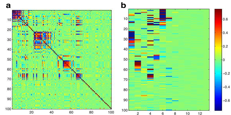
Folder: Simulations\Example_simulation contains a simulation of 100 traits from a known pedigree with low-rank genetic and residual covariances. The full covariance matrix has 8 factors, 5 of which have non-zero heritabilities. The script: ``model_setup.m" Shows how to initialize necessary parameters. Adjust this file as necessary, and then run. The script produces a figure of the posterior mean G matrix (Figure 1(a)), and the posterior mean genetic loading matrix (Figure 1(b)).
The simulations described in the accompanying paper can be generated using the R script ``generate_simulations_halfSib.R"

Figure 1: Results from Example 1. a) Posterior mean genetic covariance matrix. b) Posterior mean factor loadings.

4.2 Drosophila gene expression

Folder Ayroles_et_al_Competitive_fitness contains data from 414 genes, plus competitive fitness measured on flies from 40 lines of Drosophila melanogaster. See Ayroles et al (2009). Nat Gen. for details. In this example, competitive fitness and gene expression were not measured on the same pools of flies, so the competitive fitness data for the samples measured for gene expression is treated as missing data, as are the gene expression data for the samples measured for competitive fitness. Run the script ``model_setup.m" again, although this time, the burnin and thinning rates should probably be expanded. Figure 2 gives example output.

Figure 2: Results from Example 2 based on Drosophila expression data. a) Posterior mean genetic covariance matrix. b) Posterior mean factor loadings.

About this document ...

This document was generated using the LaTeX2HTML translator Version 2008 (1.71)

The command line arguments were:
latex2html -split 0 -show_section_numbers -local_icons -no_navigation Instructions.tex