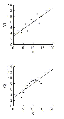
Frank Anscombe's Regression Examples
The intimate relationship between correlation and regression raises the
question of whether it is possible for a regression analysis to be misleading in
the same sense as the set of scatterplots all of which had a correlation
coefficient of 0.70. In 1973, Frank Anscombe published a set of examples showing
the answer is a definite yes (Anscombe FJ (1973), "Graphs in Statistical
Analysis," The American Statistician, 27, 17-21). Anscombe's examples share not
only the same correlation coefficient, but also the same value for any other
summary statistic that is usually calculated.

| n | 11 |
 |
9.0 |
 |
7.5 |
| Regression equation of y on x |
y = 3 + 0.5 x |
 |
110.0 |
| Regression SS | 27.5 |
| Residual SS | 13.75 (9 df) |
| Estimated SE of b1 | 0.118 |
| r | 0.816 |
| R2 | 0.667 |
 Figure 1 is the picture drawn
by the mind's eye when a simple linear regression equation is reported. Yet, the
same summary statistics apply to figure 2, which shows a perfect curvilinear
relation, and to figure 3, which shows a perfect linear relation except for a
single outlier.
The summary statistics also apply to figure 4, which is the most troublesome. Figures 2 and 3 clearly call the straight line relation into question. Figure 4 does not. A straight line may be appropriate in the fourth case. However, the regression equation is determined entirely by the single observation at x=19. Paraphrasing Anscombe, we need to know the relation between y and x and the special contribution of the observation at x=19 to that relation.
| x | y1 | y2 | y3 | x4 | y4 |
| 10 | 8.04 | 9.14 | 7.46 | 8 | 6.58 |
| 8 | 6.95 | 8.14 | 6.77 | 8 | 5.76 |
| 13 | 7.58 | 8.74 | 12.74 | 8 | 7.71 |
| 9 | 8.81 | 8.77 | 7.11 | 8 | 8.84 |
| 11 | 8.33 | 9.26 | 7.81 | 8 | 8.47 |
| 14 | 9.96 | 8.10 | 8.84 | 8 | 7.04 |
| 6 | 7.24 | 6.13 | 6.08 | 8 | 5.25 |
| 4 | 4.26 | 3.10 | 5.39 | 19 | 12.50 |
| 12 | 10.84 | 9.13 | 8.15 | 8 | 5.56 |
| 7 | 4.82 | 7.26 | 6.42 | 8 | 7.91 |
| 5 | 5.68 | 4.74 | 5.73 | 8 | 6.89 |