library("dplyr")
library("ggplot2")
library("knitr")
library("broom")
library("readr")
library("cowplot")
library("car") # for VIF function
library("STA210") # diamonds data set
set.seed(12)
diamonds <- diamonds %>% filter(carat < 1.1)
diamonds_data <- diamonds %>% sample_n(300)

## create  color dummy variables
diamonds_data <- diamonds_data %>% mutate(colorD = ifelse(color=="D",1,0),
                                colorE = ifelse(color=="E",1,0),
                                colorF = ifelse(color=="F",1,0),
                                colorG = ifelse(color=="G",1,0),
                                colorH = ifelse(color=="H",1,0),
                                colorI = ifelse(color=="I",1,0),
                                colorJ = ifelse(color=="J",1,0))

## create clarity dummy variables
diamonds_data <- diamonds_data %>% mutate(claritySI2 = ifelse(clarity=="SI2",1,0),
                                          claritySI1 = ifelse(clarity=="SI1",1,0),
                                          clarityVS2 = ifelse(clarity=="VS2",1,0),
                                          clarityVS1 = ifelse(clarity=="VS1",1,0),
                                          clarityVVS2 = ifelse(clarity=="VVS2",1,0),
                                          clarityVVS1 = ifelse(clarity=="VVS1",1,0),
                                          clarityIF = ifelse(clarity=="IF",1,0),
                                          clarityI1 = ifelse(clarity=="I1",1,0))
#add log of price
diamonds_data <- diamonds_data %>% mutate(logPrice= log(price))

# add quadractic terms and centered terms for carats
diamonds_data <- diamonds_data %>% mutate(caratCent = carat - mean(carat),
                                          caratCent.sq = caratCent^2,
                                          carat.sq = carat^2)
# original model
model.orig <- lm(logPrice ~ caratCent + caratCent.sq + colorD +
                  colorE + colorF + colorG + colorH + colorI +
                  claritySI2 + claritySI1 + clarityVS2 +
                  clarityVS1 + clarityVVS2 + clarityVVS1 +
                  clarityIF,data=diamonds_data)
# residuals plots
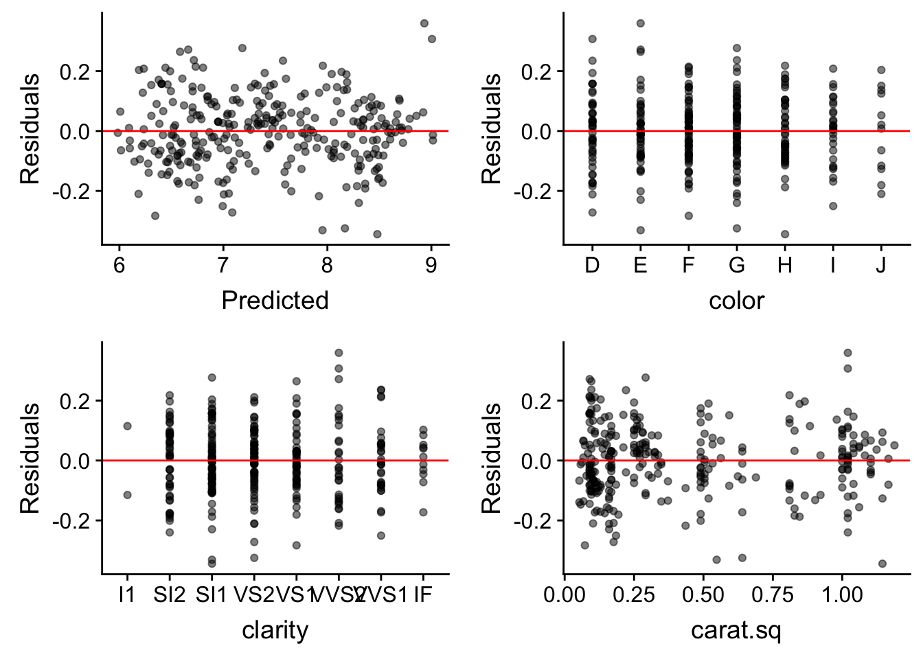
diamonds_data <- diamonds_data %>% mutate(Predicted = predict.lm(model.orig),Residuals = resid(model.orig))
p1 <-ggplot(data=diamonds_data,aes(x=Predicted,y=Residuals)) + geom_point(alpha=0.5) + geom_hline(yintercept=0,color="red")
p2 <- ggplot(data=diamonds_data,aes(x=color,y=Residuals)) + geom_point(alpha=0.5) + geom_hline(yintercept=0,color="red")
p3 <- ggplot(data=diamonds_data,aes(x=clarity,y=Residuals)) + geom_point(alpha=0.5) + geom_hline(yintercept=0,color="red")
p4 <- ggplot(data=diamonds_data,aes(x=carat.sq,y=Residuals)) + geom_point(alpha=0.5) + geom_hline(yintercept=0,color="red")
plot_grid(p1,p2,p3,p4,ncol=2)
# Is clarity important?
model.no.clarity <- lm(logPrice ~ carat + carat.sq + colorD +
                         colorE + colorF +
                         colorG + colorH + colorI,
                       data=diamonds_data)
tidy(anova(model.orig,model.no.clarity))
## # A tibble: 2 x 6
##   res.df   rss    df sumsq statistic   p.value
## *  <dbl> <dbl> <dbl> <dbl>     <dbl>     <dbl>
## 1    284  4.06    NA  NA         NA  NA
## 2    291 14.2     -7 -10.1      101.  2.42e-73
#Are there any significant interaction terms?
model.with.int <- lm(logPrice ~ carat + carat.sq + colorD + colorE +
                                    colorF + colorG + colorH + colorI +
                  claritySI2 + claritySI1 + clarityVS2 + clarityVS1 +
                    clarityVVS2 + clarityVVS1 + clarityIF + color*carat + clarity*carat,data=diamonds_data)
tidy(anova(model.orig,model.with.int))
## # A tibble: 2 x 6
##   res.df   rss    df  sumsq statistic p.value
## *  <dbl> <dbl> <dbl>  <dbl>     <dbl>   <dbl>
## 1    284  4.06    NA NA         NA     NA
## 2    271  3.83    13  0.230      1.25   0.243
#add leverage, cook's distance and standardized residuals to data set
diamonds_data <- diamonds_data %>%
  mutate(leverage = hatvalues(model.orig),
         cooks = cooks.distance(model.orig),
         stand.resid = rstandard(model.orig),
         obs.num = row_number())
#plot leverage
ggplot(data=diamonds_data, aes(x=obs.num,y=leverage)) +
  geom_point(alpha=0.5) +
  geom_hline(yintercept=0.1,color="red")+
  labs(x="Observation Number",y="Leverage",title="Leverage")

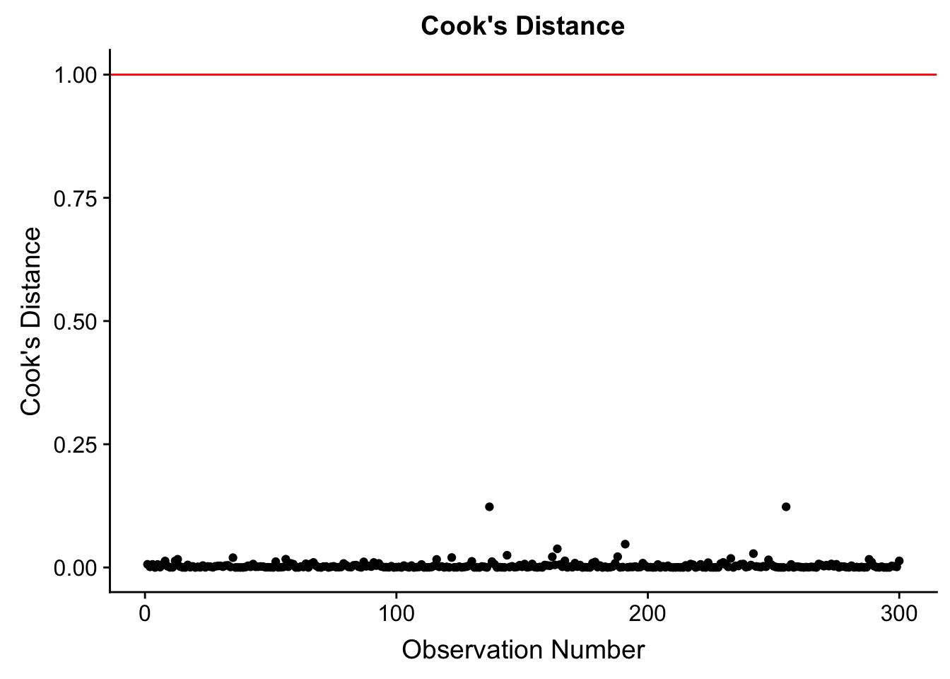
#plot cook's distance
ggplot(data=diamonds_data, aes(x=obs.num,y=cooks)) +
  geom_point() +
  geom_hline(yintercept=1,color="red")+
  labs(x="Observation Number",y="Cook's Distance",title="Cook's Distance")
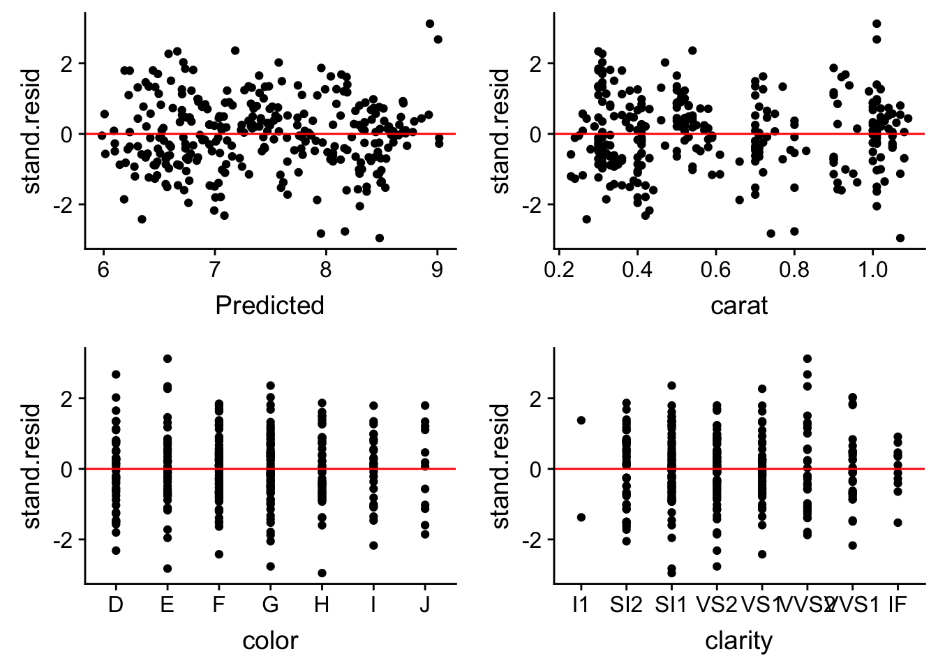
#Residuals pots using the standardized residuals
p1 <- ggplot(data=diamonds_data, aes(x=Predicted,y=stand.resid)) + geom_point()+ geom_hline(yintercept=0,color="red")
p2 <- ggplot(data=diamonds_data, aes(x=carat,y=stand.resid)) + geom_point()+ geom_hline(yintercept=0,color="red")
p3 <- ggplot(data=diamonds_data, aes(x=color,y=stand.resid)) + geom_point()+ geom_hline(yintercept=0,color="red")
p4 <- ggplot(data=diamonds_data, aes(x=clarity,y=stand.resid)) + geom_point()+ geom_hline(yintercept=0,color="red")
plot_grid(p1,p2,p3,p4,ncol=2)
#Identify high leverage points
diamonds_data %>% filter(leverage > 0.4) %>%
  select(price,color,clarity,carat)
## # A tibble: 2 x 4
##   price color clarity carat
##   <int> <ord> <ord>   <dbl>
## 1  1808 H     I1       0.96
## 2  2594 F     I1       0.94
# VIF
library(car)
tidy(vif(model.orig))
## # A tibble: 15 x 2
##    names            x
##    <chr>        <dbl>
##  1 caratCent     1.71
##  2 caratCent.sq  1.41
##  3 colorD        4.04
##  4 colorE        4.13
##  5 colorF        5.08
##  6 colorG        5.07
##  7 colorH        4.02
##  8 colorI        3.04
##  9 claritySI2   21.0
## 10 claritySI1   27.4
## 11 clarityVS2   27.0
## 12 clarityVS1   21.5
## 13 clarityVVS2  14.9
## 14 clarityVVS1  15.4
## 15 clarityIF     6.48
#Examine high VIF in clarity
diamonds_data %>% group_by(clarity) %>% summarise(n=n())
## # A tibble: 8 x 2
##   clarity     n
##   <ord>   <int>
## 1 I1          2
## 2 SI2        47
## 3 SI1        67
## 4 VS2        65
## 5 VS1        47
## 6 VVS2       30
## 7 VVS1       31
## 8 IF         11