Suggested, not to turn in. Problem 17 of Chapter 8. Data in ragwort.txt
Read in data.
Using "Data" - "Transform", create these new variables: sqrt(mass), sqrt(load), log(mass), log(load).
-
Produce a pairs plot of all pairs of X's and Y's. Under "Graph" - "2D Plot", choose "Plot Type" "Scatter Plot Matrix". Shift click for all relevant X's (load, log(load) and sqrt(load)), and all relevant Y's.
Which two plots show a linear relationship between load and mass variables?
For the best two models selected above, plot residuals vs. fitted values, and choose the best fitting model. Does your model also offer ease of interpretation? Interpret the slope parameter in a sentence.
We have two monitors for measuring indoor concentrations of carbon monoxide (CO). Each take measurements every minute. Monitor A is a newer, more accurate monitor. Monitor B is an older monitor. In a quality assurance experiment to verify that the monitors are measuring the same concentrations, both monitors co-located near a CO source, and are turned on simultaneously. The datafile, monitor.txt, gives CO concentrations (in ppm) measured by Monitor A (column 1) and Monitor B (column 2). Label the columns X and Y.
Produce a regression line plot of Y=Monitor B versus X=Monitor A. Do this using the command line:
> attach(monitor)
> par(pty="s")
> plot(X,Y, main="Comparison of New (X) and Old (Y) \n CO Monitors",xlab="Monitor A (ppm CO)", ylab="Monitor B (ppm CO)",xlim=c(0,75),ylim=c(0,75))
> abline(0,1,lty=1) # solid line, slope 1
> abline(lm(Y~X),lty=2) # dotted line, fitted regression line
Regress Y=Monitor B on X=Monitor A concentration measurements and report the fitted line.
Perform a test of whether the slope of the regression is equal to 1. Let alpha=0.05. Clearly provide test statistic, rejection region, and conclusion (Refer to HW1 Solutions, #1c, for example, for the correct format/syntax for writing out the results of a hypothesis test.).
Determine 95% confidence intervals for b0 and b1, such that the two confidence intervals simultaneously capture the slope and intercept of the regression line with 95% probability. Hint: Use the Bonferroni procedure (p. 156 of Sleuth). What do these intervals say about how well the two monitors agree (that is, does the interval for the intercept include zero, and does the interval for the slope include 1)?
We wish to predict Monitor A's measurement when Monitor B reads 20 ppm. Give a 95% prediction interval for Monitor A's measurement.
Crab claw size and force, #25 Sleuth, page 194, Ch. 7.
This data comes from: Behrens Yamada, S. and E.G. Boulding. 1998. Claw morphology, prey size selection, and foraging efficiency in generalists and specialist shell-breaking crabs. Journal of Experimental Marine Biology and Ecology 220:191-211. It can be easily downloaded from Duke E-Reserves.
Data in crabclaw.txt:
Variables: Mean closing force (Newtons) and height (mm)
Splus hints. Also review Section 8.4. Do (a), (b), (c) in the book.- Additional items:
What is the effect of a tripling of the height for the Hemigrapsus nudus?
Give a 95% confidence interval for b1 for the Hemigrapsus nudus. What are the units of b1?
-
Give a 95% confidence interval for the multiplicative factor in the median for the Hemigrapsus nudus.
For each crab, closing forces were measured repeatedly, by measuring the force as the claws pulled two wires together. Could this be considered an ecological regression? Why or why not? Are their any other statistics besides the mean that might be appropriate to measure closing force?
Risk and Sammarco found that the skeletal density of the coral Porites lobata increases with distance from the Australian shore due to differences between inshore and offshore environments. The dataset, reef.txt, provides the following data for the density of Great Barrier Reef coral heads:
- Sample
- Reef Name
- Distance to shore (km)
- Coral head density (g/cm
3 )
-
Produce a regression line plot of Y=coral head density vs. X=distance to shore.
-
Report the fitted regression line. In one sentence each, interpret the slope, intercept and R2. (Look under "Example - Big Bang" on p. 173 for an example of such interpretations, and also refer to HW1 solutions for the format/syntax here.)
Assess lack of fit of the linear regression model by a plot of residuals vs. fitted values.
Assess lack of fit of the linear regression model using the lack of fit F-test.
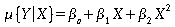
Investigating a polynomial fit. We will now consider the following regression model:
- First, make a plot of this fitted model for the coral reef data. Go to "Graph" - "2D Plot" - "Fit-Polynomial Curvefit". Choose the X and Y variables as before. Click on the "Curve Fitting" tab and check that you are fitting "Curve Fit Type: Linear" and "Poly. Order 2". Click "OK" to produce the plot.
- Next, fit the model by choosing "Statistics" - "Regression" - "Linear". In the "Formula" box, type "Density~Distance+Distance^2". Write out the fitted model.
- In the regression output for the fitted model, look at the p-value corresponding to "I(Distance^2)". This is the p-value for the two-sided hypothesis test of Ho: b2 = 0 in the presence of b0 and b1. That is, we are comparing the simple linear model to the polynomial model of degree 2. What does the p-value say about the polynomial model?