Time Series

# Time Series
### Dr. Maria Tackett
### 04.22.19

---

### Announcements

- Project write up due May 1 at 2p

- Project presentations on May 1
    - Lab 01L: 2p - 3:30p
    - Lab 02L: 3:30p - 5p
    
- Exam 2 grades by next Monday

- Exam 2 extra credit: If the response rate for the course evaluations is 90%, everyone gets +1 pt on their Exam 2 score (out of 40 pts)

---

## Examples of Time Series Data

---

## Gas Prices in Durham
 
.center[
<img src="img/23/durham-gas-price.png" width="90%" style="display: block; margin: auto;" />

[https://www.gasbuddy.com/Charts](https://www.gasbuddy.com/Charts)
]

---

## Apple's Stock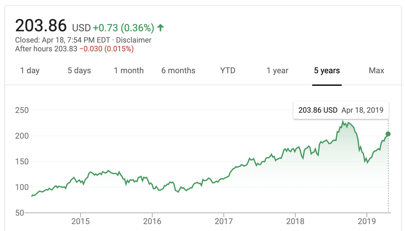

[Apple's Stock Price](https://www.google.com/search?rlz=1C5CHFA_enUS812US814&tbm=fin&q=NASDAQ:+AAPL&stick=H4sIAAAAAAAAAONgecRoyi3w8sc9YSmdSWtOXmNU4-IKzsgvd80rySypFJLgYoOy-KR4uLj0c_UNzKtyk8rSeADviEaCOgAAAA&biw=1219&bih=1169#scso=_zp_YW7edDdGxggeTqLqYCw1:0)

]
---

## Google Music Timeline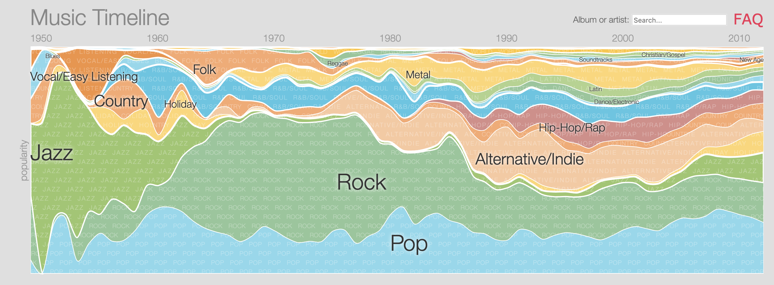

[http://research.google.com/bigpicture/music/](http://research.google.com/bigpicture/music/)
]

---

## Today's Example

---

## Bike rentals in DC

- <font class="vocab">Goal:</font> To predict the number of bike rentals in the Capital BikeShare. We'll use the 2012 data
<br>

---

## Bike Rentals vs. Temperature

- In a previous analysis, we used temperature to predict number of bike rentals.

<img src="23-time-series_files/figure-html/unnamed-chunk-4-1.png" style="display: block; margin: auto;" />
  
---

## Bike Rentals vs. Temperature

<table>
 <thead>
  <tr>
   <th style="text-align:left;"> term </th>
   <th style="text-align:right;"> estimate </th>
   <th style="text-align:right;"> std.error </th>
   <th style="text-align:right;"> statistic </th>
   <th style="text-align:right;"> p.value </th>
  </tr>
 </thead>
<tbody>
  <tr>
   <td style="text-align:left;"> (Intercept) </td>
   <td style="text-align:right;"> -18446.639 </td>
   <td style="text-align:right;"> 1716.251 </td>
   <td style="text-align:right;"> -10.748 </td>
   <td style="text-align:right;"> 0 </td>
  </tr>
  <tr>
   <td style="text-align:left;"> temp_f </td>
   <td style="text-align:right;"> 616.346 </td>
   <td style="text-align:right;"> 50.879 </td>
   <td style="text-align:right;"> 12.114 </td>
   <td style="text-align:right;"> 0 </td>
  </tr>
  <tr>
   <td style="text-align:left;"> temp_f_sq </td>
   <td style="text-align:right;"> -3.753 </td>
   <td style="text-align:right;"> 0.367 </td>
   <td style="text-align:right;"> -10.223 </td>
   <td style="text-align:right;"> 0 </td>
  </tr>
</tbody>
</table>

There is evidence that the independence assumption is violated, i.e. there is **serial correlation**
---

## Time Series

- One assumption for the regression methods we've used so far is that the observations are independent of one another
    + In other words, the residuals are independent 
--

- When data is ordered over time, errors in one time period may influence error in another time period

- We'll use <font class = "vocab">time series analysis</font> to deal with this serial correlation
    + Assume the observations are measured at equally spaced time points

- Today's class is a brief introduction to time series analysis
  + You can take *STA 444: Statistical Modeling of Spatial and Time Series Data* for more in-depth study of the subject

---

## Autocorrelation

- We want a measure of the correlation between the observation at time `$t$` and the observation at time `$t-k$`
    + `$k$` is the **lag**

- To do so, we will compute the correlation between the observations (or  residuals) at time `$t$` and time `$t-k$`
    - This is the **autocorrelation coefficient**

- The formula for the <font class="vocab">Lag <i>k</i> autocorrelation coefficient is </font>

`$$r_k = \frac{\sum\limits_{i=1}^{n-k}(y_i - \bar{y})(y_{i+k} - \bar{y})}{\sum\limits_{i=1}^n (y_i - \bar{y})^2}$$`

---

## Bikeshare rentals

```r
bike <- bike %>%
  mutate(cnt_lag_1 = lag(cnt, n = 1), 
         cnt_lag_2 = lag(cnt, n = 2))
```

```
## # A tibble: 5 x 3
##     cnt cnt_lag_1 cnt_lag_2
##   <int>     <int>     <int>
## 1  2294        NA        NA
## 2  1951      2294        NA
## 3  2236      1951      2294
## 4  2368      2236      1951
## 5  3272      2368      2236
```

---

### Bikeshare: autocorrelation

- We can use the <font class="vocab">`acf()`</font> function to calculate the autocorrelation coefficient

```r
orig_acf <- acf(bike$cnt, plot = F)$acf
orig_acf[2] #lag 1 autocorrelation
```

```
## [1] 0.7483672
```

---

## Autoregressive Model

- There are many models that can be used to account for serial correlation

- Common model is the <font class="vocab">autoregressive (AR) model</font>

- If we have no predictor variables, the AR model with one lag, the <font class="vocab3">AR(1) model</font>, is

`$$y_t = \beta_0 + \beta_1 y_{t-1} + \epsilon_t \hspace{10mm} \epsilon_t \sim N(0,\sigma^2)$$`

---

### Bikeshare: AR(1) Model

```r
ar_1_model <- lm(cnt ~ cnt_lag_1, data = bike)
```

<table>
 <thead>
  <tr>
   <th style="text-align:left;"> term </th>
   <th style="text-align:right;"> estimate </th>
   <th style="text-align:right;"> std.error </th>
   <th style="text-align:right;"> statistic </th>
   <th style="text-align:right;"> p.value </th>
  </tr>
 </thead>
<tbody>
  <tr>
   <td style="text-align:left;"> (Intercept) </td>
   <td style="text-align:right;"> 1382.510 </td>
   <td style="text-align:right;"> 202.437 </td>
   <td style="text-align:right;"> 6.829 </td>
   <td style="text-align:right;"> 0 </td>
  </tr>
  <tr>
   <td style="text-align:left;"> cnt_lag_1 </td>
   <td style="text-align:right;"> 0.754 </td>
   <td style="text-align:right;"> 0.034 </td>
   <td style="text-align:right;"> 21.907 </td>
   <td style="text-align:right;"> 0 </td>
  </tr>
</tbody>
</table>

- **Slope**: For each additional bike rental on day `$t-1$`, we expect there to be about 0.754 bike rentals on day `$t$`.

- **Intercept**: If there are 0 bike rentals on day `$t-1$`, we expect there to be about 1383 bike rentals on day `$t$`.
    - Not meaningful in practice

---

## Residual Plots

```r
ar_1_aug <- augment(ar_1_model) %>% 
  mutate(dteday = bike$dteday[2:nrow(bike)])
```

---

## Residual Plots

---

## Autocorrelation

- We can use the residuals to calculate autocorrelation to see if the AR(1) model is an appropriate fit for the data

```r
ar1_acf <- acf(ar_1_aug$.resid, plot = FALSE)$acf
ar1_acf[2] #lag 1 autocorrelation
```

```
## [1] -0.1276273
```

- This is a significant improvement on the autocorrelation! But is there still significant autocorrelation?

---

## ACF Plot

- We can use an <font class = "vocab">autocorrelation function (ACF) plot</font> to see the autocorrelation at different lags

- Generally, if the line extends outside of the blue dotted lines, there is  potentially significant autocorrelation between observations at time `$t$` and time `$t-k$`

```r
acf(ar_1_aug$.resid, plot = TRUE, main = "ACF of Residuals after AR(1) Model")
```

---

## ACF Plot

```r
acf(ar_1_aug$.resid, plot = TRUE, main = "ACF of Residuals after AR(1) Model")$acf[2]
```

```
## [1] -0.1276273
```

- Autocorrelation is much lower, but can we reduce it further?

---

### Try AR(2) Model

```r
ar_2_model <- lm(cnt ~ cnt_lag_1 + cnt_lag_2, data = bike[-2,])
kable(tidy(ar_2_model), format = "html", digits = 3)
```

<table>
 <thead>
  <tr>
   <th style="text-align:left;"> term </th>
   <th style="text-align:right;"> estimate </th>
   <th style="text-align:right;"> std.error </th>
   <th style="text-align:right;"> statistic </th>
   <th style="text-align:right;"> p.value </th>
  </tr>
 </thead>
<tbody>
  <tr>
   <td style="text-align:left;"> (Intercept) </td>
   <td style="text-align:right;"> 1173.303 </td>
   <td style="text-align:right;"> 213.817 </td>
   <td style="text-align:right;"> 5.487 </td>
   <td style="text-align:right;"> 0.000 </td>
  </tr>
  <tr>
   <td style="text-align:left;"> cnt_lag_1 </td>
   <td style="text-align:right;"> 0.626 </td>
   <td style="text-align:right;"> 0.052 </td>
   <td style="text-align:right;"> 12.078 </td>
   <td style="text-align:right;"> 0.000 </td>
  </tr>
  <tr>
   <td style="text-align:left;"> cnt_lag_2 </td>
   <td style="text-align:right;"> 0.165 </td>
   <td style="text-align:right;"> 0.052 </td>
   <td style="text-align:right;"> 3.186 </td>
   <td style="text-align:right;"> 0.002 </td>
  </tr>
</tbody>
</table>

---

## ACF Plot

```
## [1] -0.02139348
```

This autocorrelation looks good!

---

## Add `temp` and `workingday`

- Look at the data in the **Time Series** RStudio Cloud project

---

## Futher Reading

- [*Time Series Analysis and Its Applications*](https://www.stat.pitt.edu/stoffer/tsa4/tsa4.pdf) by Shumway and Stoffer
    - graduate-level text

- [*Time Series: A Data Analysis Approach*](https://www.stat.pitt.edu/stoffer/tsda/) by Shumway and Stoffer 
    - introductory text
    - published May 2019