class: center, middle, inverse, title-slide # (tidy)Text analysis ### Yue Jiang ### 02.12.20 --- layout: true <div class="my-footer"> <span> <a href="http://datasciencebox.org" target="_blank">datasciencebox.org</a> </span> </div> --- ## Announcements - R Workshop tomorrow -- get your questions in! - Exam - Today's application exercise --- class: center, middle # Tidytext analysis --- ## Packages In addition to `tidyverse` we will be using a few other packages today ```r library(tidyverse) library(tidytext) library(genius) # https://github.com/JosiahParry/genius library(wordcloud) library(reshape2) ``` --- ## Tidytext - Using tidy data principles can make many text mining tasks easier, more effective, and consistent with tools already in wide use. - Learn more at https://www.tidytextmining.com/. --- ## What is tidy text? ```r text <- c("On your mark ready set let's go", "dance floor pro", "I know you know I go psycho", "When my new joint hit", "just can't sit", "Got to get jiggy wit it", "ooh, that's it") text ``` ``` ## [1] "On your mark ready set let's go" "dance floor pro" ## [3] "I know you know I go psycho" "When my new joint hit" ## [5] "just can't sit" "Got to get jiggy wit it" ## [7] "ooh, that's it" ``` --- ## What is tidy text? ```r text_df <- tibble(line = 1:7, text = text) text_df ``` ``` ## # A tibble: 7 x 2 ## line text ## <int> <chr> ## 1 1 On your mark ready set let's go ## 2 2 dance floor pro ## 3 3 I know you know I go psycho ## 4 4 When my new joint hit ## 5 5 just can't sit ## 6 6 Got to get jiggy wit it ## 7 7 ooh, that's it ``` --- ## What is tidy text? ```r text_df %>% unnest_tokens(word, text) ``` ``` ## # A tibble: 34 x 2 ## line word ## <int> <chr> ## 1 1 on ## 2 1 your ## 3 1 mark ## 4 1 ready ## 5 1 set ## 6 1 let's ## 7 1 go ## 8 2 dance ## 9 2 floor ## 10 2 pro ## # ... with 24 more rows ``` --- ## Let's get some data We'll use the `genius` package to get song lyric data from [Genius](https://genius.com/). - `genius_album()` allows you to download the lyrics for an entire album in a tidy format. - Input: Two arguments: artist and album. Supply the quoted name of artist and the album (if it gives you issues check that you have the album name and artists as specified on [Genius](https://genius.com/)). - Output: A tidy data frame with three columns corresponding to the track name, the track number, and lyrics ```r ariana <- genius_album( artist = "Ariana Grande", album = "thank you, next" ) national <- genius_album( artist = "The National", album = "I Am Easy to Find" ) ``` --- ## Ariana Grande vs. The National .pull-left[ <img src="img/07/ariana.png" width="90%" /> ] .pull-right[ <img src="img/07/national.png" width="90%" /> ] --- ## Save for later ```r ariana <- ariana %>% mutate( artist = "Ariana Grande", album = "thank you, next" ) national <- national %>% mutate( artist = "The National", album = "I Am Easy to Find" ) ``` --- ## What songs are in the album? <small> ```r ariana %>% distinct(track_title) ``` ``` ## # A tibble: 12 x 1 ## track_title ## <chr> ## 1 <U+200B>imagine ## 2 <U+200B>needy ## 3 NASA ## 4 <U+200B>bloodline ## 5 <U+200B>fake smile ## 6 <U+200B>bad idea ## 7 <U+200B>make up ## 8 <U+200B>ghostin ## 9 <U+200B>in my head ## 10 7 rings ## 11 <U+200B>thank u, next ## 12 <U+200B>break up with your girlfriend, i'm bored ``` </small> --- ## What songs are in the album? <small> ```r national %>% distinct(track_title) ``` ``` ## # A tibble: 16 x 1 ## track_title ## <chr> ## 1 You Had Your Soul with You (Ft. Gail Ann Dorsey) ## 2 Quiet Light ## 3 Roman Holiday ## 4 Oblivions ## 5 The Pull of You ## 6 Hey Rosey ## 7 I Am Easy to Find ## 8 Her Father in the Pool ## 9 Where Is Her Head ## 10 Not in Kansas ## 11 So Far So Fast ## 12 Dust Swirls in Strange Light ## 13 Hairpin Turns ## 14 Rylan ## 15 Underwater ## 16 Light Years ``` </small> --- ## Tidy up your lyrics! ```r ariana_lyrics <- ariana %>% unnest_tokens(word, lyric) national_lyrics <- national %>% unnest_tokens(word, lyric) ``` --- ## What are the most common words? .pull-left[ ```r ariana_lyrics %>% count(word) %>% arrange(desc(n)) ``` ``` ## # A tibble: 685 x 2 ## word n ## <chr> <int> ## 1 i 241 ## 2 you 232 ## 3 yeah 194 ## 4 it 163 ## 5 a 89 ## 6 i'm 86 ## 7 me 83 ## 8 the 76 ## 9 and 74 ## 10 my 71 ## # ... with 675 more rows ``` ] .pull-right[ ```r national_lyrics %>% count(word) %>% arrange(desc(n)) ``` ``` ## # A tibble: 710 x 2 ## word n ## <chr> <int> ## 1 i 184 ## 2 you 143 ## 3 the 126 ## 4 to 90 ## 5 me 75 ## 6 and 74 ## 7 is 68 ## 8 in 60 ## 9 a 58 ## 10 i'm 53 ## # ... with 700 more rows ``` ] --- ## Stop words - In computing, stop words are words which are filtered out before or after processing of natural language data (text). - They usually refer to the most common words in a language, but there is not a single list of stop words used by all natural language processing tools. See `?get_stopwords` for more info. ```r get_stopwords(source = "smart") ``` ``` ## # A tibble: 571 x 2 ## word lexicon ## <chr> <chr> ## 1 a smart ## 2 a's smart ## 3 able smart ## 4 about smart ## 5 above smart ## 6 according smart ## 7 accordingly smart ## 8 across smart ## 9 actually smart ## 10 after smart ## # ... with 561 more rows ``` --- ## What are the most common words? .pull-left[ ```r ariana_lyrics %>% anti_join(get_stopwords(source = "smart")) %>% count(word) %>% arrange(desc(n)) ``` ``` ## # A tibble: 458 x 2 ## word n ## <chr> <int> ## 1 yeah 194 ## 2 eh 42 ## 3 love 41 ## 4 i'ma 37 ## 5 girlfriend 31 ## 6 imagine 30 ## 7 forget 27 ## 8 make 24 ## 9 space 24 ## 10 bad 19 ## # ... with 448 more rows ``` ] .pull-right[ ```r national_lyrics %>% anti_join(get_stopwords(source = "smart")) %>% count(word) %>% arrange(desc(n)) ``` ``` ## # A tibble: 488 x 2 ## word n ## <chr> <int> ## 1 time 20 ## 2 eyes 15 ## 3 light 13 ## 4 learning 12 ## 5 lightyears 12 ## 6 hands 11 ## 7 head 11 ## 8 quiet 11 ## 9 standing 11 ## 10 feeling 10 ## # ... with 478 more rows ``` ] --- ## What are the most common words? ```r ariana_lyrics %>% anti_join(get_stopwords(source = "smart")) %>% count(word) %>% arrange(desc(n)) %>% top_n(20) %>% ggplot(aes(fct_reorder(word, n), n)) + geom_col() + coord_flip() + theme_minimal() + labs(title = "Frequency of 'thank u, next' lyrics", y = "", x = "") ``` --- ## What are the most common words? <!-- --> --- ## What are the most common words? <!-- --> --- ## Sentiment analysis - One way to analyze the sentiment of a text is to consider the text as a combination of its individual words - The sentiment content of the whole text as the sum of the sentiment content of the individual words - The sentiment attached to each word is given by a *lexicon*, which may be downloaded from external sources --- ## Sentiment lexicons .pull-left[ ```r get_sentiments("afinn") ``` ``` ## # A tibble: 2,477 x 2 ## word value ## <chr> <dbl> ## 1 abandon -2 ## 2 abandoned -2 ## 3 abandons -2 ## 4 abducted -2 ## 5 abduction -2 ## 6 abductions -2 ## 7 abhor -3 ## 8 abhorred -3 ## 9 abhorrent -3 ## 10 abhors -3 ## # ... with 2,467 more rows ``` ] .pull-right[ ```r get_sentiments("bing") ``` ``` ## # A tibble: 6,786 x 2 ## word sentiment ## <chr> <chr> ## 1 2-faces negative ## 2 abnormal negative ## 3 abolish negative ## 4 abominable negative ## 5 abominably negative ## 6 abominate negative ## 7 abomination negative ## 8 abort negative ## 9 aborted negative ## 10 aborts negative ## # ... with 6,776 more rows ``` ] --- ## Sentiment lexicons .pull-left[ ```r get_sentiments("nrc") ``` ``` ## # A tibble: 13,901 x 2 ## word sentiment ## <chr> <chr> ## 1 abacus trust ## 2 abandon fear ## 3 abandon negative ## 4 abandon sadness ## 5 abandoned anger ## 6 abandoned fear ## 7 abandoned negative ## 8 abandoned sadness ## 9 abandonment anger ## 10 abandonment fear ## # ... with 13,891 more rows ``` ] .pull-right[ ```r get_sentiments("loughran") ``` ``` ## # A tibble: 4,150 x 2 ## word sentiment ## <chr> <chr> ## 1 abandon negative ## 2 abandoned negative ## 3 abandoning negative ## 4 abandonment negative ## 5 abandonments negative ## 6 abandons negative ## 7 abdicated negative ## 8 abdicates negative ## 9 abdicating negative ## 10 abdication negative ## # ... with 4,140 more rows ``` ] --- ## Notes about sentiment lexicons - Not every word is in a lexicon! ```r get_sentiments("bing") %>% filter(word == "data") ``` ``` ## # A tibble: 0 x 2 ## # ... with 2 variables: word <chr>, sentiment <chr> ``` - Lexicons do not account for qualifiers before a word (e.g., "not happy") because they were constructed for one-word tokens only - Summing up each word's sentiment may result in a neutral sentiment, even if there are strong positive and negative sentiments in the body --- ## Sentiments in lyrics .pull-left[ ```r ariana_lyrics %>% inner_join(get_sentiments("bing")) %>% count(sentiment, word) %>% arrange(desc(n)) ``` ``` ## # A tibble: 95 x 3 ## sentiment word n ## <chr> <chr> <int> ## 1 positive like 45 ## 2 positive love 41 ## 3 positive thank 39 ## 4 negative bad 19 ## 5 positive good 19 ## 6 positive smile 17 ## 7 negative fake 16 ## 8 positive woo 13 ## 9 negative shit 11 ## 10 positive right 11 ## # ... with 85 more rows ``` ] .pull-right[ ```r national_lyrics %>% inner_join(get_sentiments("bing")) %>% count(sentiment, word) %>% arrange(desc(n)) ``` ``` ## # A tibble: 90 x 3 ## sentiment word n ## <chr> <chr> <int> ## 1 positive like 14 ## 2 positive quiet 11 ## 3 positive easy 9 ## 4 negative fear 8 ## 5 negative dust 7 ## 6 negative hate 7 ## 7 negative lie 7 ## 8 negative strange 7 ## 9 positive fast 7 ## 10 negative hard 6 ## # ... with 80 more rows ``` ] --- ## Visualizing sentiments ```r ariana_lyrics %>% inner_join(get_sentiments("bing")) %>% count(sentiment, word) %>% arrange(desc(n)) %>% group_by(sentiment) %>% top_n(10) %>% ungroup() %>% ggplot(aes(fct_reorder(word, n), n, fill = sentiment)) + geom_col() + coord_flip() + facet_wrap(~ sentiment, scales = "free_y") + theme_minimal() + labs(title = "Sentiments in Ariana Lyrics", x = "") ``` --- ## Visualizing sentiments <!-- --> --- ## Visualizing sentiments <!-- --> --- ## Ariana word cloud ```r library(wordcloud) set.seed(12345) ariana_lyrics %>% anti_join(stop_words) %>% count(word) %>% with(wordcloud(word, n, max.words = 100)) ``` --- ## Ariana word cloud <!-- --> --- ## The National word cloud <!-- --> --- ## Word frequencies, Ariana vs. The National ```r # combine the lyrics, calculate frequencies combined <- bind_rows(ariana_lyrics, national_lyrics) %>% anti_join(get_stopwords(source = "smart")) %>% group_by(artist) %>% count(word, sort = T) %>% mutate(freq = n / sum(n)) %>% select(artist, word, freq) %>% spread(artist, freq) # make into nice plot ggplot(combined, aes(x = `Ariana Grande`, y = `The National`))+ # hide discreteness geom_jitter(alpha = 0.1, size = 2.5, width = 0.25, height = 0.25) + geom_text(aes(label = word), check_overlap = T, vjust = 1.5)+ scale_x_log10()+ scale_y_log10()+ geom_abline(color = "blue") ``` --- ## Word frequencies, Ariana vs. The National 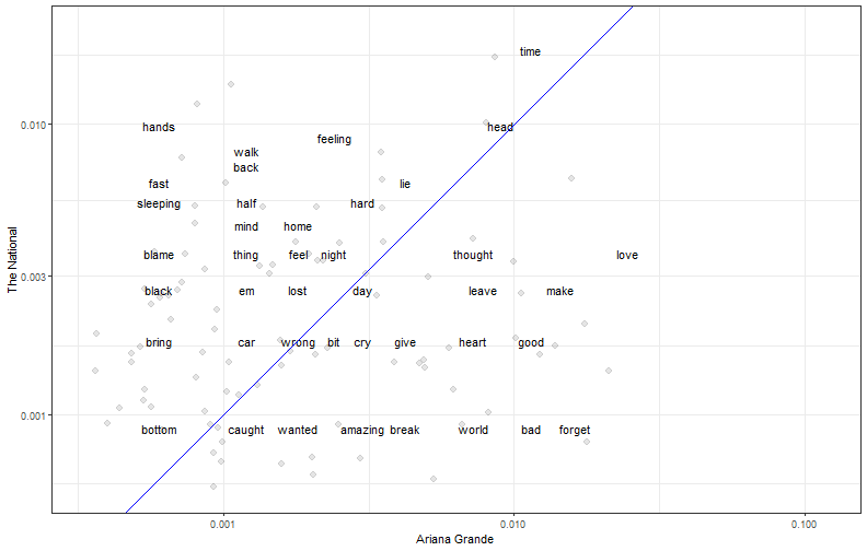<!-- --> --- ## On your own Application Exercise, available at [https://classroom.github.com/a/hPdnIAFI](https://classroom.github.com/a/hPdnIAFI)