class: center, middle, inverse, title-slide # Logistic Regression (2) ### Yue Jiang ### STA 210 / Duke University / Spring 2024 --- ### Logistic Regression model `$$\text{log}\left(\frac{p_i}{1-p_i}\right) = \beta_0 + \beta_1 x_{i1} + \beta_2 x_{i2} + \cdots + \beta_p x_{ip}$$` `$$E(y_i | x_{i1}, \cdots, x_{ip}) = p_i = \frac{e^{\beta_0 + \beta_1 x_{i1} + \beta_2 x_{i2} + \cdots + \beta_p x_{ip}}}{1 + e^{\beta_0 + \beta_1 x_{i1} + \beta_2 x_{i2} + \cdots + \beta_p x_{ip}}}$$` --- ### Interpreting "slope" parameters We often like to interpret things as **odds ratios**, not as log-odds (what is -2.1 log-odds of success, anyway?). Holding all other variables in the model constant, each one unit increase in `\(x_k\)` is *associated with* an `\(e^{\beta_k}\)` multiplicative factor on the odds of success. That is, in comparing two individuals one unit apart in `\(x_k\)` (while holding the other predictors constant), the individual with the one unit higher `\(x_k\)` is *predicted to have* `\(e^{\beta_k}\)` times the odds of success compared to the other. .question[ The wording above was for a continuous predictor. How might you adapt it for categorical predictors? ] --- ### Today's data <br><br>  --- ### A model ```r pokemon <- read.csv("data/pokemon.csv") m1 <- glm(Legendary ~ HP + Attack + Defense + Sp..Atk + Sp..Def + Speed, data = pokemon, family = "binomial") summary(m1) ``` --- ### A model ``` ## ## Call: ## glm(formula = Legendary ~ HP + Attack + Defense + Sp..Atk + Sp..Def + ## Speed, family = "binomial", data = pokemon) ## ## Deviance Residuals: ## Min 1Q Median 3Q Max ## -2.325 -0.293 -0.104 -0.019 4.708 ## ## Coefficients: ## Estimate Std. Error z value Pr(>|z|) ## (Intercept) -16.94852 1.30293 -13.01 < 0.0000000000000002 *** ## HP 0.03468 0.00530 6.54 0.00000000006093 *** ## Attack 0.01367 0.00455 3.00 0.0027 ** ## Defense 0.03155 0.00530 5.95 0.00000000270521 *** ## Sp..Atk 0.02827 0.00447 6.32 0.00000000025411 *** ## Sp..Def 0.02493 0.00555 4.49 0.00000705446411 *** ## Speed 0.03805 0.00526 7.24 0.00000000000046 *** ## --- ## Signif. codes: 0 '***' 0.001 '**' 0.01 '*' 0.05 '.' 0.1 ' ' 1 ## ## (Dispersion parameter for binomial family taken to be 1) ## ## Null deviance: 837.59 on 1189 degrees of freedom ## Residual deviance: 418.22 on 1183 degrees of freedom ## AIC: 432.2 ## ## Number of Fisher Scoring iterations: 7 ``` --- ### A model ```r library(tidymodels) m1_aug <- augment(m1) m1_aug ``` ``` ## # A tibble: 1,190 x 13 ## Legend~1 HP Attack Defense Sp..Atk Sp..Def Speed .fitted .resid .std.r~2 ## <int> <int> <int> <int> <int> <int> <int> <dbl> <dbl> <dbl> ## 1 0 45 49 49 65 65 45 -8.00 -0.0259 -0.0259 ## 2 0 60 62 63 80 80 60 -5.49 -0.0906 -0.0906 ## 3 0 80 82 83 100 100 80 -2.07 -0.487 -0.488 ## 4 0 39 52 43 60 50 65 -8.11 -0.0245 -0.0245 ## 5 0 58 64 58 80 65 80 -5.31 -0.0995 -0.0995 ## 6 0 78 84 78 109 85 100 -1.63 -0.599 -0.600 ## 7 0 44 48 65 50 64 43 -8.07 -0.0250 -0.0250 ## 8 0 59 63 80 65 80 58 -5.48 -0.0913 -0.0913 ## 9 0 79 83 100 85 105 78 -1.93 -0.520 -0.521 ## 10 0 45 30 35 20 20 45 -11.1 -0.00551 -0.00551 ## # ... with 1,180 more rows, 3 more variables: .hat <dbl>, .sigma <dbl>, ## # .cooksd <dbl>, and abbreviated variable names 1: Legendary, 2: .std.resid ``` --- ### Classification Logistic regression allows us to obtain predicted probabilities of success for a binary variable. By imposing a threshold (for example if the probability is greater than 0.5) we can create a classifier. - Logistic regression has assumptions: independence and linearity in the log-odds (more on this in just a bit) - Straightforward interpretation of coefficients - Handles numerical and categorical predictors - Can quantify uncertainty around a prediction --- ### From log-odds to probabilities ```r m1_aug <- m1_aug %>% mutate(prob = exp(.fitted)/(1 + exp(.fitted)), pred_leg = ifelse(prob > 0.5, "Legendary", "Not Legendary")) %>% select(.fitted, prob, pred_leg, Legendary) ``` --- ### Some hypothetical Pokemon Suppose we have the following hypothetical Pokemon. How would we classify them using our model? (HP / ATK / DEF / SPA / SPD / SPE) - Crapistat: 55 / 25 / 30 / 60 / 50 / 102 - Mediocra: 90 / 90 / 130 / 75 / 80 / 45 - This is literally Dragonite: 91 / 134 / 95 / 100 / 100 / 80 - Broaken: 110 / 125 / 105 / 148 / 102 / 136 ```r tidy(m1) ``` ``` ## # A tibble: 7 x 5 ## term estimate std.error statistic p.value ## <chr> <dbl> <dbl> <dbl> <dbl> ## 1 (Intercept) -16.9 1.30 -13.0 1.10e-38 ## 2 HP 0.0347 0.00530 6.54 6.09e-11 ## 3 Attack 0.0137 0.00455 3.00 2.67e- 3 ## 4 Defense 0.0316 0.00530 5.95 2.71e- 9 ## 5 Sp..Atk 0.0283 0.00447 6.32 2.54e-10 ## 6 Sp..Def 0.0249 0.00555 4.49 7.05e- 6 ## 7 Speed 0.0381 0.00526 7.24 4.56e-13 ``` --- ### Some hypothetical Pokemon ```r new_pokemon <- tibble(HP = c(55, 90, 91, 104), Attack = c(25, 110, 134, 125), Defense = c(30, 130, 95, 105), Sp..Atk = c(60, 75, 100, 148), Sp..Def = c(50, 80, 100, 102), Speed = c(102, 45, 80, 136)) pred_log_odds <- augment(m1, newdata = new_pokemon) %>% pull(.fitted) pred_probs <- exp(pred_log_odds)/(1 + exp(pred_log_odds)) round(pred_probs, 3) ``` ``` ## [1] 0.001 0.084 0.354 0.973 ``` --- ### How well did we predict? ```r table(m1_aug$pred_leg, m1_aug$Legendary) ``` ``` ## ## 0 1 ## Legendary 24 69 ## Not Legendary 1032 65 ``` --- ### Binary classifiers Suppose we're interested in the performance of a binary classifier. Let `\(A\)` be the event that an observation is "positive" (e.g., legendary), and let `\(B\)` be the event that a classifier for that condition *says* positive (e.g., *predicted* to be legendary) - .vocab[Prevalence]: `\(P(A)\)` The proportion of individuals with the condition - .vocab[Sensitivity]: `\(P(B|A)\)`, or the true positive rate - .vocab[Specificity]: `\(P(B^c|A^c)\)`, or 1 minus the false positive rate - .vocab[Positive Predictive Value]: `\(P(A|B)\)` - .vocab[Negative Predictive Value]: `\(P(A^c|B^c)\)` .question[ What do these probabilities mean in plain English? ] --- ### "False positives" ``` ## [1] "Slaking" "Hydreigon" ## [3] "Venusaur Mega Venusaur" "Charizard Mega Charizard X" ## [5] "Charizard Mega Charizard Y" "Blastoise Mega Blastoise" ## [7] "Alakazam Mega Alakazam" "Gengar Mega Gengar" ## [9] "Gyarados Mega Gyarados" "Aerodactyl Mega Aerodactyl" ## [11] "Houndoom Mega Houndoom" "Tyranitar Mega Tyranitar" ## [13] "Sceptile Mega Sceptile" "Blaziken Mega Blaziken" ## [15] "Swampert Mega Swampert" "Gardevoir Mega Gardevoir" ## [17] "Aggron Mega Aggron" "Salamence Mega Salamence" ## [19] "Metagross Mega Metagross" "Garchomp Mega Garchomp" ## [21] "Lucario Mega Lucario" "Greninja Ash-Greninja" ## [23] "Dragapult" "Palafin Hero Form" ``` --- ### "False negatives" ``` ## [1] "Articuno" "Zapdos" ## [3] "Moltres" "Raikou" ## [5] "Entei" "Suicune" ## [7] "Regirock" "Regice" ## [9] "Registeel" "Deoxys Normal Forme" ## [11] "Deoxys Attack Forme" "Uxie" ## [13] "Mesprit" "Azelf" ## [15] "Phione" "Cobalion" ## [17] "Terrakion" "Virizion" ## [19] "Tornadus Incarnate Forme" "Tornadus Therian Forme" ## [21] "Thundurus Incarnate Forme" "Thundurus Therian Forme" ## [23] "Landorus Incarnate Forme" "Landorus Therian Forme" ## [25] "Genesect" "Diancie" ## [27] "Hoopa Hoopa Confined" "Volcanion" ## [29] "Zygarde10% Forme" "Type: Null" ## [31] "Silvally" "Tapu Koko" ## [33] "Tapu Lele" "Tapu Bulu" ## [35] "Tapu Fini" "Cosmog" ## [37] "Cosmoem" "Nihilego" ## [39] "Buzzwole" "Pheromosa" ## [41] "Xurkitree" "Celesteela" ## [43] "Kartana" "Guzzlord" ## [45] "Necrozma" "Magearna" ## [47] "Marshadow" "Poipole" ## [49] "Naganadel" "Stakataka" ## [51] "Blacephalon" "Meltan" ## [53] "Melmetal" "Kubfu" ## [55] "Urshifu Single Strike Style" "Urshifu Rapid Strike Style" ## [57] "Zarude" "Glastrier" ## [59] "Calyrex" "Enamorus Incarnate Forme" ## [61] "Enamorus Therian Forme" "Ting-Lu" ## [63] "Chien-Pao" "Wo-Chien" ## [65] "Chi-Yu" ``` --- ### Discrimination thresholds We can classify Pokemon as legendary ("positive") or non-legendary ("negative") depending on a continuous value - the predicted probability of legendary status. - If the predicted probability is above a certain threshold, it is classified as legendary - Varying the threshold for a positive vs. negative test will result in a test in different characteristics - But should this threshold be that classifies Pokemon as legendary? - At each threshold value, there is a trade-off between sensitivity and specificity .question[ Can you come up with a naive example of a "perfectly sensitive" classifier? Would the classifier you come up with be good in practice? ] --- ### ROC curves .copper[Receiver Operating Characteristic] curves show how specificity and specificity change as the discrimination threshold changes <img src="img/radar1.jpg" width="80%" style="display: block; margin: auto;" /> --- ### ROC curves ```r m1_aug %>% sample_n(20) ``` ``` ## .fitted prob pred_leg Legendary pokemon$Name ## 1 -7.0706 0.0008490 Not Legendary 0 Tyrunt ## 2 -8.7145 0.0001642 Not Legendary 0 Deino ## 3 -3.6480 0.0253817 Not Legendary 0 Flapple ## 4 -4.1004 0.0162964 Not Legendary 0 Audino ## 5 0.0119 0.5029764 Legendary 0 Blaziken Mega Blaziken ## 6 -3.2205 0.0384007 Not Legendary 0 Bewear ## 7 -9.0663 0.0001155 Not Legendary 0 Chewtle ## 8 0.7024 0.6687112 Legendary 1 Deoxys Speed Forme ## 9 -7.5659 0.0005175 Not Legendary 0 Pumpkaboo Small Size ## 10 -2.2220 0.0977945 Not Legendary 0 Flygon ## 11 -9.3362 0.0000882 Not Legendary 0 Marill ## 12 -5.1947 0.0055153 Not Legendary 0 Arctibax ## 13 -0.9063 0.2877499 Not Legendary 0 Great Tusk ## 14 0.0494 0.5123555 Legendary 1 Regidrago ## 15 -2.3498 0.0870810 Not Legendary 0 Klinklang ## 16 -3.1409 0.0414529 Not Legendary 0 Barraskewda ## 17 -10.9508 0.0000175 Not Legendary 0 Poochyena ## 18 -1.9653 0.1228983 Not Legendary 0 Mandibuzz ## 19 -8.2695 0.0002562 Not Legendary 0 Turtwig ## 20 -5.8211 0.0029555 Not Legendary 0 Combusken ``` --- ### ROC curves ```r m1_aug %>% roc_curve( truth = as.factor(Legendary), prob, event_level = "second" ) ``` ``` ## # A tibble: 1,124 x 3 ## .threshold specificity sensitivity ## <dbl> <dbl> <dbl> ## 1 -Inf 0 1 ## 2 0.00000740 0 1 ## 3 0.00000845 0.000947 1 ## 4 0.00000884 0.00189 1 ## 5 0.00000888 0.00284 1 ## 6 0.00000922 0.00379 1 ## 7 0.0000117 0.00473 1 ## 8 0.0000118 0.00568 1 ## 9 0.0000139 0.00663 1 ## 10 0.0000140 0.00758 1 ## # ... with 1,114 more rows ``` --- ### ROC curves ```r m1_aug %>% roc_curve( truth = as.factor(Legendary), prob, event_level = "second" ) %>% autoplot() ``` <!-- --> --- ### The area under the ROC curve ```r m1_aug %>% roc_auc( truth = as.factor(Legendary), prob, event_level = "second" ) ``` ``` ## # A tibble: 1 x 3 ## .metric .estimator .estimate ## <chr> <chr> <dbl> ## 1 roc_auc binary 0.942 ``` The .vocab[AUC] (area under the curve) can be used to assess how well we are predicting, and summarizes the entire ROC curve. An AUC of 0.5 implies that the model is no better than a coin flip - an AUC of 1 implies a perfect fit. The AUC also represents the probability that a randomly selected legendary ("positive") Pokemon has a higher estimated score (in this case, the predicted probability) than that of a randomly selected non-legendary ("negative") Pokemon. --- ### Assumptions If you do some Googling, you'll find all sorts of "assumptions" for logistic regression. Many of these assumptions are just "nice things to have" and aren't actually necessary. The only two assumptions we'll be talking about are .vocab[independence] and .vocab[linearity] (well, some notion of "linearity" anyway). - .vocab[Independence]: the *observations* are independent from each other (careful - *not* the predictors) - .vocab[Linearity]: there is a linear relationship between the log-odds of the response and the predictors --- ### Perfect separation What if all legendary Pokemon were water type? What would the odds ratio be for odds of being a legendary Pokemon comparing water vs. non-water Pokemon? --- ### Empirical logits The .vocab[empirical logit] is given by the following: `\begin{align*} \log\left(\frac{\# Yes~(Legendary)}{\# No~(Non-legendary)}\right) \end{align*}` --- ### Empirical logistics (continuous predictors) ```r library(Stat2Data) emplogitplot1(Legendary ~ HP, data = pokemon, ngroups = 10) ``` 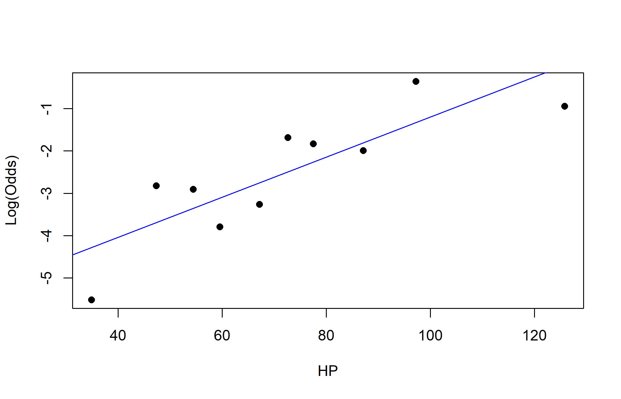<!-- --> --- ### Empirical logits (continuous predictors) ```r emplogitplot1(Legendary ~ Attack, data = pokemon, ngroups = 10) ``` 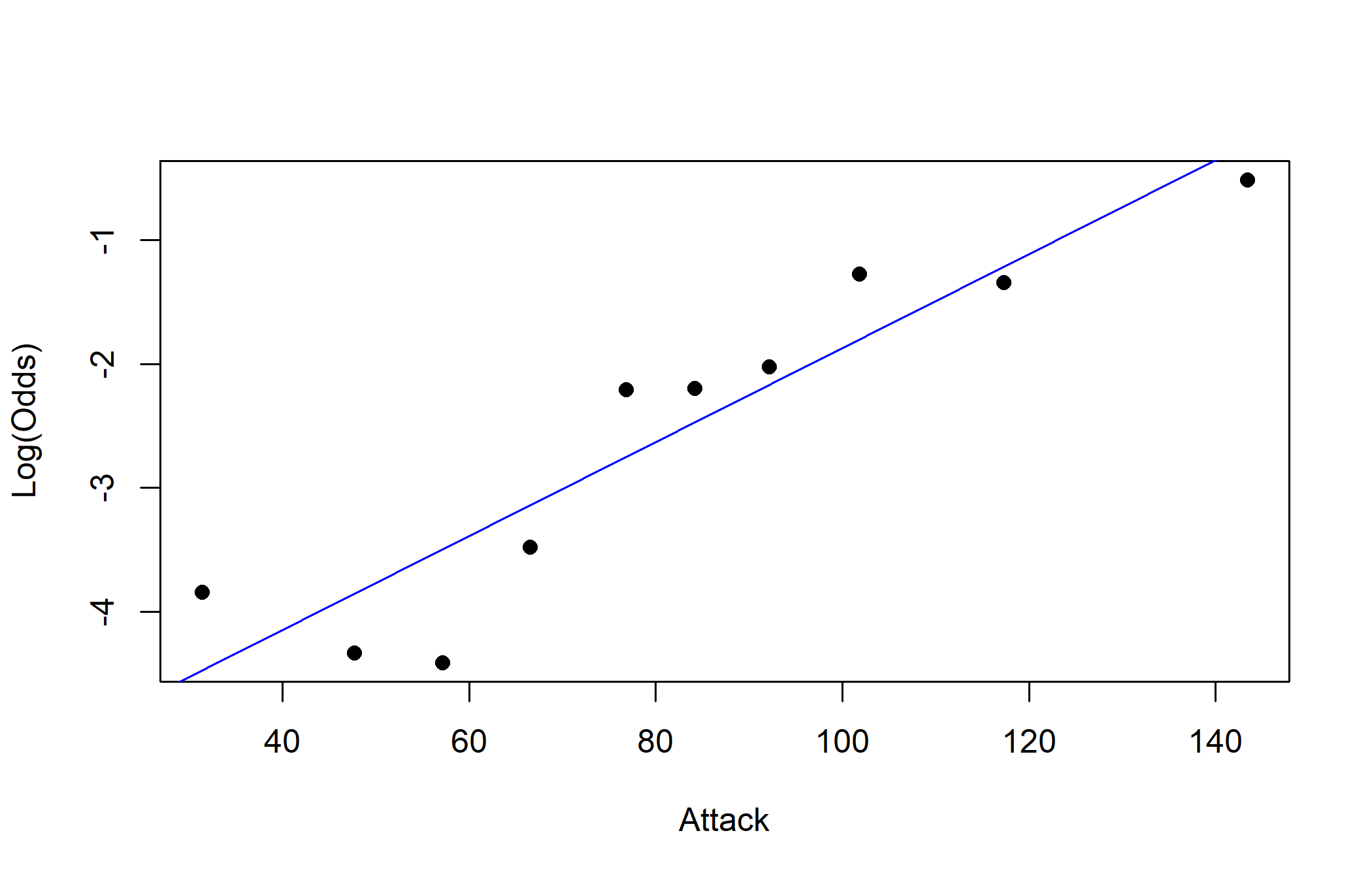<!-- --> --- ### Empirical logits (continuous predictors) ```r emplogitplot1(Legendary ~ Speed, data = pokemon, ngroups = 10) ``` 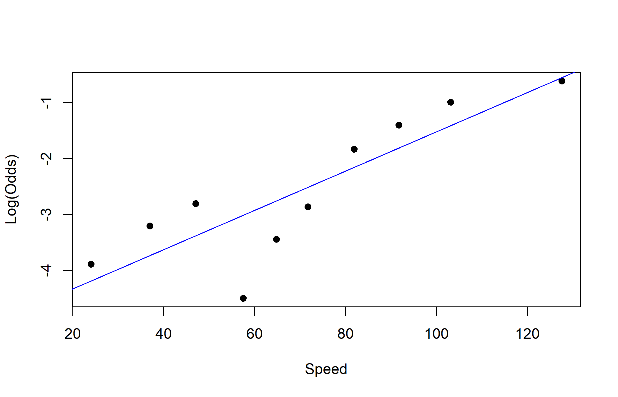<!-- --> --- <br><br><br><br><br>