class: center, middle, inverse, title-slide # Data visualization workshop ### Yue Jiang ### Duke University / STA 583 / Spring 2024 --- ## Why do we visualize? Below is an excerpt from the `datasaurus_dozen` dataset: ``` ## # A tibble: 13 x 2 ## dataset r ## <chr> <dbl> ## 1 away -0.0641 ## 2 bullseye -0.0686 ## 3 circle -0.0683 ## 4 dino -0.0645 ## 5 dots -0.0603 ## 6 h_lines -0.0617 ## 7 high_lines -0.0685 ## 8 slant_down -0.0690 ## 9 slant_up -0.0686 ## 10 star -0.0630 ## 11 v_lines -0.0694 ## 12 wide_lines -0.0666 ## 13 x_shape -0.0656 ``` --- ## Why do we visualize? .question[ How similar do the relationships between `x` and `y` look based on the plots? Based on the summary statistics? ] 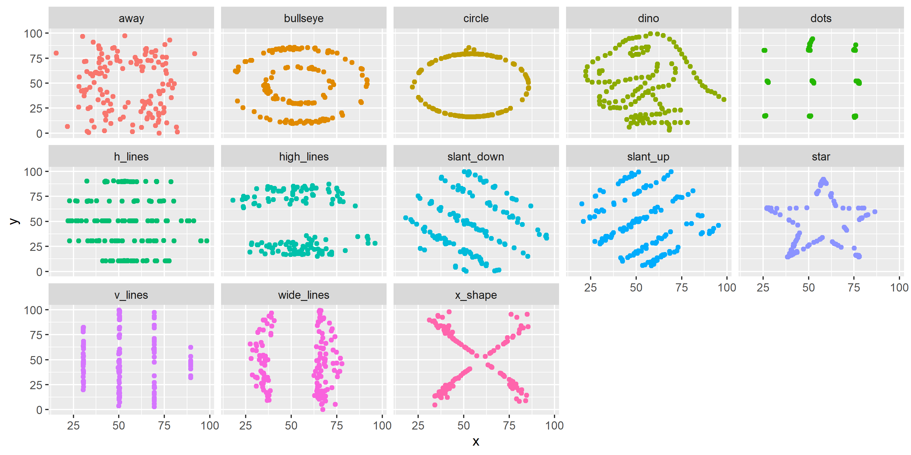<!-- --> --- ## Anscombe's quartet ```r library(Tmisc) quartet ``` .pull-left[ ``` ## set x y ## 1 I 10 8.04 ## 2 I 8 6.95 ## 3 I 13 7.58 ## 4 I 9 8.81 ## 5 I 11 8.33 ## 6 I 14 9.96 ## 7 I 6 7.24 ## 8 I 4 4.26 ## 9 I 12 10.84 ## 10 I 7 4.82 ## 11 I 5 5.68 ## 12 II 10 9.14 ## 13 II 8 8.14 ## 14 II 13 8.74 ## 15 II 9 8.77 ## 16 II 11 9.26 ## 17 II 14 8.10 ## 18 II 6 6.13 ## 19 II 4 3.10 ## 20 II 12 9.13 ## 21 II 7 7.26 ## 22 II 5 4.74 ``` ] .pull-right[ ``` ## set x y ## 23 III 10 7.46 ## 24 III 8 6.77 ## 25 III 13 12.74 ## 26 III 9 7.11 ## 27 III 11 7.81 ## 28 III 14 8.84 ## 29 III 6 6.08 ## 30 III 4 5.39 ## 31 III 12 8.15 ## 32 III 7 6.42 ## 33 III 5 5.73 ## 34 IV 8 6.58 ## 35 IV 8 5.76 ## 36 IV 8 7.71 ## 37 IV 8 8.84 ## 38 IV 8 8.47 ## 39 IV 8 7.04 ## 40 IV 8 5.25 ## 41 IV 19 12.50 ## 42 IV 8 5.56 ## 43 IV 8 7.91 ## 44 IV 8 6.89 ``` ] --- ## Summarising Anscombe's quartet ```r quartet %>% group_by(set) %>% summarise( mean_x = mean(x), mean_y = mean(y), sd_x = sd(x), sd_y = sd(y), r = cor(x, y) ) ``` ``` ## # A tibble: 4 x 6 ## set mean_x mean_y sd_x sd_y r ## <fct> <dbl> <dbl> <dbl> <dbl> <dbl> ## 1 I 9 7.50 3.32 2.03 0.816 ## 2 II 9 7.50 3.32 2.03 0.816 ## 3 III 9 7.5 3.32 2.03 0.816 ## 4 IV 9 7.50 3.32 2.03 0.817 ``` --- ## Visualizing Anscombe's quartet ```r ggplot(quartet, aes(x = x, y = y)) + geom_point() + facet_wrap(~ set, ncol = 4) ``` <!-- --> --- ## Keep it simple <img src="img/04/pie-3d.jpg" width="300" style="display: block; margin: auto;" /> <img src="lec-4_files/figure-html/pie-to-bar-1.png" width="600" style="display: block; margin: auto;" /> --- ## Use color to draw attention <img src="lec-4_files/figure-html/unnamed-chunk-1-1.png" width="500" style="display: block; margin: auto;" /> <img src="lec-4_files/figure-html/unnamed-chunk-2-1.png" width="600" style="display: block; margin: auto;" /> --- ## Tell a story <img src="img/04/time-series.story.png" width="800" style="display: block; margin: auto;" /> .footnote[ Credit: Angela Zoss and Eric Monson, Duke DVS ] --- ### Some effective visualizations [An amazing website!](http://r-statistics.co/Top50-Ggplot2-Visualizations-MasterList-R-Code.html) --- ### In-class activity