Practice Final Exam

1. Assume that GPA's at a particular university are normally distributed with a mean of 3.0, a median of 3.3, and a standard deviation of 0.5.

a) (6 pts) What would be the percentile rank for a student with a GPA of 3.4?







b) (3 pts) What can you say about the shape of the distribution of GPA's

2. (6 pts) A researcher randomly picks 100 phone numbers from a city phone book. She then calls each number and asks the person who answers to come in for a paid research study. Ninety percent of those called show up for the study. In the study, she takes the first 45 subjects and gives them an experimental drug designed to improve memory, and then gives them a memory test. For the next 45 subjects who show up, she gives them an inert sugar pill, and gives them a memory test. Circle all of the adjectives below that describe this study:

double-blind placebo-controlled simple random sample

random assignment to groups observational experimental

3. (6 pts) The Sheriff of Nottingham is taking some badly needed archery practice. He shoots at the target 200 times, and has a probability of hitting the taret of 0.6 with each shot. The shots are independent. What is the chance that he will hit the target at least 135 times?

4. (6 pts) The mean annual income for a random sample of 25 women receiving food stamps is $9,768, with a standard deviation of $2,125. Calculate the 95% confidence interval for the true mean income of the population of women receiving food stamps.
   
   
   
   
   


5. Consider the following probabilities:

i) The probability, if H₀ is false, that you will reject H₀.

ii) The probability, computed assuming that H₀ is true, of getting a test statistic as extreme as that actually observed.

iii) The probability that H₀ is true.

iv) The probability, computed assuming that H₀ is true, that you will reject H₀.

v) The probability that H₀ is true given the extreme value of the observed statistic.

vi) The probability, if H₀ is false, that you will retain H₀.

(Only one answer from above is to be given to each question below.)

a) (2 pts) Which of the above corresponds to a?

b) (2 pts) Which corresponds to b?

c) (2 pts) Which corresponds to power?

d) (2 pts) Which corresponds to a p-value?

6. (6 pts) The Ozarski Corporation, a bicycle maker, obtains tires from three suppliers: the Field Company, the Otley Company, and the West Company. During 1997, the Ozarski Corporation received the following numbers of acceptable and defective tires from each supplier:

Supplier	Acceptable	Defective
Field	940	89
Otley	780	32
West	870	60

Is there a statistically significant relationship between Tire Supplier and the Acceptable/Defective variable? Use a=.05.

7. (2 pts each) True or False?

____ a) The narrower the confidence interval is, the more confident we are that it contains the population parameter.

____ b) A way to make the confidence interval narrower is to change the confidence level from 95% to 99%.

____ c) Assume the null hypothesis is H₀: m=0. If the null hypothesis is not rejected, then the corresponding confidence interval (e.g., the 95% confidence interval would correspond to an hypothesis test with a = .05) will contain the value 0.

____ d) Studies with higher statistical power will tend to have wider confidence intervals.

8. A researcher is analyzing crime data from the 50 states. Below is JMP-In output comparing murder rates across four U.S. geographical regions-- Midwest, Northeast, South, and West.

Murder By Region

Oneway Anova

Source DF Sum of Squares Mean Square F Ratio
Model 3 _________ 90.3719 ______
Error ___ _________ 10.3876 Prob>F
Total ___ 748.94420 0.0001

Alpha= 0.05

Comparisons for all pairs using Tukey-Kramer HSD

Abs(Dif)-LSD South West Northeast Midwest
South -3.03732 1.16772 1.57118 2.08391
West 1.16772 -3.36960 -2.95002 -2.44998
Northeast 1.57118 -2.95002 -4.04976 -3.57431
Midwest 2.08391 -2.44998 -3.57431 -3.50719

Positive values show pairs of means that are significantly different.

a) (5 pts) Fill in the blanks in the ANOVA summary table.

b) (5 pts) Interpret, in terms of the variables given in the problem, the overall ANOVA results.

c) (5 pts) Interpret the results of the pairwise comparisons.

9. (6 pts) Suppose an employee in San Francisco needs to call any one of five colleagues at home. Assume that the 5 colleagues are random selections from a population and that 21.5% of San Francisco numbers are unlisted. Find the probability that at least one of the five fellow workers will have a listed phone number.

10. Below is JMP-In output showing the relationship between unemployment rates and auto theft rates (annual rate per 100,000 autos) across the 50 states.

Auto By Unemployment

Linear Fit

Auto = 112.137 + 56.7802 Unemployment

Summary of Fit

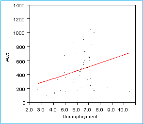
RSquare 0.108613
Root Mean Square Error 252.4688
Mean of Response 473.6
Observations (or Sum Wgts) 50

Parameter Estimates

Term Estimate Std Error t Ratio Prob>|t|
Intercept 112.13722 153.6689 0.73 0.4691
Unemployment 56.780205 23.47839 2.42 0.0194

a) (3 pts) Interpret the slope of the regression equation.

b) (3 pts) Interpret Root Mean Square Error

c) (3 pts) Is unemployment a significant predictor of auto theft?

d) (3 pts) What would you predict the auto theft rate would be for a state with an unemployment rate of 7.5?

e) (3 pts) Can we conclude that higher unemployment causes higher auto theft rates? Why or why not?

11. (6 pts) Suppose that 0.5% (.005) of all students seeking treatment at a school infirmary are eventually diagnosed as having mononucleosis. Of those who do have mono, 90% complain of a sore throat. But 30% of those not having mono also have sore throats. If a student comes to the infirmary and says that he has a sore throat, what is the probability that he has mono?