11-1

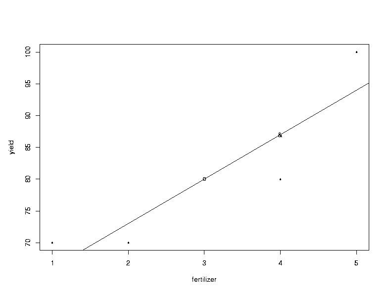
1. For the given data, [`X] = 3, [`Y] = 80, åxy = 70 and åx² = 10, so that

   b = å xy å x2 = 70 10 = 7 a = _ Y   - b _ X   = 80-7·3 = 59 ,

   and the estimated regression line is

   ^ Y   = 59 + 7 X .

2. Here is the graphic. The only points of interest here are the ones marked with a ``·'' .

   

3. 1. [^Y] = 59+7·3 = 80; this corresponds to the point marked with an ``o'' in the previous graph.
   2. [^Y] = 59+7·4 = 87; this corresponds to the point marked with an ``&'' in the previous graph.
   3. This corresponds to the estimated slope of the regression line, b = 7.

11-3

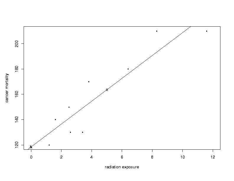
1. Here, b = åxy /åx² = 876/97 » 9.031 and a = [`Y]-b[`X] » 160 - 9.031·4.6 = 118.457, so that the estimated regression line is [^Y] = 118.457 + 9.031 X.
2. For a radiation exposure of 5.0, we estimate the cancer mortality to be [^Y] = 118.457 + 9.031·5 = 163.612. For a radiation exposure of zero, the estimated cancer mortality is the estimated intercept, a = 118.457.
3. The answer to b. with zero exposure is marked with an ``&'', the answer to part b. with exposure 5.0 with an ``o'' and the counties with a ``·''.

   

4. Since the data arises from an uncontroled observational study, one can not conclude for any causal relationship between radiation exposure and cancer mortality. It can be the case that the observed positive relation between the two variables is due to the presence of some confounding variable.

11-5