Homework #6--Suggested Answers
ISBE 6.1, 6.3, 6.6, 6.11, 6.12 6.15, 6.19
6.1
- $1,475,113. Of the sample, resale was about 21% of the
total dollar value (1,475,113 represents approximately 21% of the value
of all 552,000 orders).
- We had to assume that those who responded were representative of the
population of customers. This would not be the case if the ratio of
the number of resalers to personal users was very different in the
sample and in the population (are resalers more likely to respond?).
It would also not be the case if a customer's choice to respond to
the survey depended on the dollar value of his/her purchases (are big
spenders more likely to respond?). Differential response rates will
lead to biases in estimates called nonresponse bias.
- $95,882.32. This is amount for resale ($1,475,112.68) times
the tax rate (0.065).
6.3
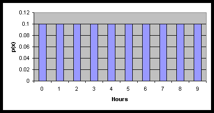
a.

b. 3, 6, 7, 4, 4
c. m
= 4.5
d. The sample mean is closer to m
than many of the individual observations.
6.6
- $800. SE = 8,000/Square root of 100
- Since the standard deviation and sample size remain the same, the standard error would be the same.
6.11
- 4.7%. SE is .12, thus the Z score is -1.67.
- <.000483. SE is .06, thus the Z score is -3.333.
- Approximately 0. SE is .03, thus the Z score is -6.67.
6.15
Twice. We know that as n increases the standard error decreases.
Since SE = the square root of p
(1-p
)/ n, and we know that n = 1000 for LA and 250 for San Diego, then the
denominator of SE is twice as large for LA than San Diego (square root
of 1000 = 32, SR or 250 = 16)--standard deviation will be half the size.
Thus estimates of p will be twice as
accurate.
6.19
0.00668%. We need to know Pr(P<0.5). This can be found by
assuming that P is approximately normally distributed
(1000*(1-p)>5 with
p>1/2, so this assumption is
a valid one). Begin by calculating the Z score. The standard error of
P, SE(P) = square root of .539(1-.539)/1000 = 0.015763217. Next, we
evaluate the Z score: Z =(.5-.539)/.015763217 = -2.47. Using
Table IV we find this equals P>.5 = .007 or 0.7%.

